377:
200:
97:
230:
220:
23:
210:
458:
448:
117:
438:
428:
387:
107:
127:
34:
problem is defined under the limits of initial and boundary conditions. When constructing a staggered grid, it is common to implement boundary conditions by adding an extra node across the physical boundary. The nodes just outside the inlet of the system are used to assign the inlet conditions and
35:
the physical boundaries can coincide with the scalar control volume boundaries. This makes it possible to introduce the boundary conditions and achieve discrete equations for nodes near the boundaries with small modifications.
577:
472:
The equations are solved for cells up to NI-1, outside the domain values of flow variables are determined by extrapolation from the interior by assuming zero gradients at the outlet plane
327:
280:
361:
Values of each variable at the nodes at upstream and downstream of the inlet plane are equal to values at the nodes at upstream and downstream of the outlet plane.
161:
In this type of situations values of properties just adjacent to the solution domain are taken as values at the nearest node just inside the domain.
601:
17:
76:
For the first u, v, φ-cell all links to neighboring nodes are active, so there is no need of any modifications to discretion equations.
484:
469:
In fully developed flow no changes occurs in flow direction, gradient of all variables except pressure are zero in flow direction
447:
398:
These conditions are used when we don’t know the exact details of flow distribution but boundary values of pressure are known
116:
606:
83:
40:
31:
437:
376:
199:
427:
386:
86:
codes estimate k and ε with approximate formulate based on turbulent intensity between 1 and 6% and length scale
476:
229:
219:
106:
96:
209:
457:
126:
358:
We take flux of flow leaving the outlet cycle boundary equal to the flux entering the inlet cycle boundary
336:
The velocity is constant along parallel to the wall and varies only in the direction normal to the wall.
298:
251:
79:
At one of the inlet node absolute pressure is fixed and made pressure correction to zero at that node.
22:
343:
242:
595:
289:
180:
401:
For example: external flows around objects, internal flows with multiple outlets,
402:
189:
In this we are applying the “wall functions” instead of the mesh points.
588:
An introduction to computational fluid dynamics by
Versteeg, PEARSON.
418:
Considering the case of an outlet perpendicular to the x-direction -
456:
446:
436:
426:
385:
375:
228:
218:
208:
198:
125:
115:
105:
95:
21:
72:
Consider the case of an inlet perpendicular to the x direction.
572:{\displaystyle U_{NI,J}=U_{NI-1,J}{\frac {M_{in}}{M_{out}}}\,}
183:
and the velocity varies linearly with distance from the wall
169:
Consider situation solid wall parallel to the x-direction:
487:
409:
The pressure corrections are taken zero at the nodes.
301:
285:
in the log-law region of a turbulent boundary layer.
254:
451:
Fig. 14 pressure correction cell at an exit boundary
571:
321:
274:
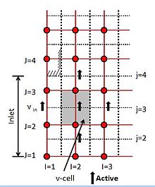
120:Fig.4 pressure correction cell at intake boundary
332:Important points for applying wall functions:
8:
441:Fig. 13 v-control volume at an exit boundary
339:No pressure gradients in the flow direction.
203:Fig.6 u-velocity cell at a physical boundary
39:The most common boundary conditions used in
431:Fig.12 A control volume at an exit boundary
568:
554:
541:
535:
514:
492:
486:
318:
306:
300:
271:
259:
253:
173:Assumptions made and relations considered
405:-driven flows, free surface flows, etc.
233:Fig.9 scalar cell at a physical boundary
110:Fig.3 v-velocity cell at intake boundary
100:Fig.2 u-velocity cell at intake boundary
156:Scalar flux across the boundary is zero
461:Fig.15 scalar cell at an exit boundary
223:Fig.8 v-cell at physical boundary j=NJ
475:The outlet plane velocities with the
213:Fig.7 v-cell at physical boundary j=3
130:Fig. 5 scalar cell at intake boundary
18:Boundary conditions in fluid dynamics
7:
380:Fig.10 p’-cell at an intake boundary
179:The near wall flow is considered as
390:Fig. 11 p’-cell at an exit boundary
147:If flow across the boundary is zero
152:Normal velocities are set to zero
14:
348:No chemical reactions at the wall
322:{\displaystyle y^{+}<11.63\,}
275:{\displaystyle y^{+}>11.63\,}
26:Fig 1 Formation of grid in cfd
1:
186:No slip condition: u = v = 0.
602:Computational fluid dynamics
165:Physical boundary conditions
84:computational fluid dynamics
54:Physical boundary conditions
41:computational fluid dynamics
32:computational fluid dynamics
366:Pressure boundary condition
142:Symmetry boundary condition
623:
68:Intake boundary conditions
15:
353:Cyclic boundary condition
414:Exit boundary conditions
573:
462:
452:
442:
432:
391:
381:
323:
276:
234:
224:
214:
204:
131:
121:
111:
101:
27:
574:
460:
450:
440:
430:
389:
379:
324:
277:
232:
222:
212:
202:
129:
119:
109:
99:
25:
485:
299:
252:
607:Boundary conditions
422:
371:
194:
91:
60:Pressure conditions
51:Symmetry conditions
569:
463:
453:
443:
433:
421:
392:
382:
370:
319:
272:
235:
225:
215:
205:
193:
132:
122:
112:
102:
90:
28:
566:
467:
466:
396:
395:
239:
238:
136:
135:
57:Cyclic conditions
48:Intake conditions
614:
578:
576:
575:
570:
567:
565:
564:
549:
548:
536:
534:
533:
506:
505:
423:
420:
372:
369:
328:
326:
325:
320:
311:
310:
281:
279:
278:
273:
264:
263:
195:
192:
92:
89:
622:
621:
617:
616:
615:
613:
612:
611:
592:
591:
585:
550:
537:
510:
488:
483:
482:
416:
368:
355:
344:Reynolds number
302:
297:
296:
255:
250:
249:
167:
144:
138:
70:
63:Exit conditions
20:
12:
11:
5:
620:
618:
610:
609:
604:
594:
593:
590:
589:
584:
581:
563:
560:
557:
553:
547:
544:
540:
532:
529:
526:
523:
520:
517:
513:
509:
504:
501:
498:
495:
491:
465:
464:
454:
444:
434:
415:
412:
411:
410:
394:
393:
383:
367:
364:
363:
362:
359:
354:
351:
350:
349:
346:
340:
337:
317:
314:
309:
305:
270:
267:
262:
258:
243:Turbulent flow
237:
236:
226:
216:
206:
191:
190:
187:
184:
166:
163:
143:
140:
134:
133:
123:
113:
103:
88:
87:
80:
77:
69:
66:
65:
64:
61:
58:
55:
52:
49:
16:Main article:
13:
10:
9:
6:
4:
3:
2:
619:
608:
605:
603:
600:
599:
597:
587:
586:
582:
580:
561:
558:
555:
551:
545:
542:
538:
530:
527:
524:
521:
518:
515:
511:
507:
502:
499:
496:
493:
489:
480:
478:
473:
470:
459:
455:
449:
445:
439:
435:
429:
425:
424:
419:
413:
408:
407:
406:
404:
399:
388:
384:
378:
374:
373:
365:
360:
357:
356:
352:
347:
345:
341:
338:
335:
334:
333:
330:
315:
312:
307:
303:
294:
292:
291:
286:
283:
268:
265:
260:
256:
247:
245:
244:
231:
227:
221:
217:
211:
207:
201:
197:
196:
188:
185:
182:
178:
177:
176:
174:
170:
164:
162:
159:
157:
153:
150:
148:
141:
139:
128:
124:
118:
114:
108:
104:
98:
94:
93:
85:
81:
78:
75:
74:
73:
67:
62:
59:
56:
53:
50:
47:
46:
45:
44:
42:
36:
33:
30:Almost every
24:
19:
481:
474:
471:
468:
417:
400:
397:
331:
295:
290:Laminar flow
288:
287:
284:
248:
241:
240:
172:
171:
168:
160:
155:
154:
151:
146:
145:
137:
71:
38:
37:
29:
479:correction
596:Categories
583:References
477:continuity
82:Generally
522:−
403:buoyancy
293: :
181:laminar
342:High
316:11.63
269:11.63
313:<
266:>
43:are
598::
579:.
329:.
282:.
246::
175:-
158::
149::
562:t
559:u
556:o
552:M
546:n
543:i
539:M
531:J
528:,
525:1
519:I
516:N
512:U
508:=
503:J
500:,
497:I
494:N
490:U
308:+
304:y
261:+
257:y
Text is available under the Creative Commons Attribution-ShareAlike License. Additional terms may apply.