862:
17:
476:. This is defined as the fraction of the measurements which can be arbitrarily changed without causing the resulting estimate to tend to infinity (i.e., to "break down"). The breakdown point of an L-estimator is given by the closest order statistic to the minimum or maximum: for instance, the median has a breakdown point of 50% (the highest possible), and a
737:
While L-estimators are not as efficient as other statistics, they often have reasonably high relative efficiency, and show that a large fraction of the information used in estimation can be obtained using only a few points – as few as one, two, or three. Alternatively, they show that order statistics
795:
gives a reasonably efficient estimator, though instead taking the 7% trimmed range (the difference between the 7th and 93rd percentiles) and dividing by 3 (corresponding to 86% of the data of a normal distribution falling within 1.5 standard deviations of the mean) yields an estimate of about 65%
788:(average of median and midhinge) can be used, though the average of the 20th, 50th, and 80th percentile yields 88% efficiency. Using further points yield higher efficiency, though it is notable that only 3 points are needed for very high efficiency.
784:), but a more efficient estimate is the 29% trimmed mid-range, that is, averaging the two values 29% of the way in from the smallest and the largest values: the 29th and 71st percentiles; this has an efficiency of about 81%. For three points, the
491:
Not all L-estimators are robust; if it includes the minimum or maximum, then it has a breakdown point of 0. These non-robust L-estimators include the minimum, maximum, mean, and mid-range. The trimmed equivalents are robust, however.
686:
L-estimators can also be used as statistics in their own right – for example, the median is a measure of location, and the IQR is a measure of dispersion. In these cases, the sample statistics can act as estimators of their own
764:
However, for a large data set (over 100 points) from a symmetric population, the mean can be estimated reasonably efficiently relative to the best estimate by L-estimators. Using a single point, this is done by taking the
673:
710:, these provided a useful way to extract much of the information from a sample with minimal labour. These remained in practical use through the early and mid 20th century, when automated sorting of
799:
For small samples, L-estimators are also relatively efficient: the midsummary of the 3rd point from each end has an efficiency around 84% for samples of size about 10, and the range divided by
366:
151:
91:
are preferred, although these are much more difficult computationally. In many circumstances L-estimators are reasonably efficient, and thus adequate for initial estimation.
821:
729:, and the X% trimmed mid-range has an X% breakdown point, while the sample mean (which is maximally efficient) is minimally robust, breaking down for a single outlier.
225:
702:
Assuming sorted data, L-estimators involving only a few points can be calculated with far fewer mathematical operations than efficient estimates. Before the advent of
265:
186:
294:
460:
are L-estimators for the population L-moment, and have rather complex expressions. L-moments are generally treated separately; see that article for details.
75:: assuming sorted data, they are very easy to calculate and interpret, and are often resistant to outliers. They thus are useful in robust statistics, as
68:
of the measurements. This can be as little as a single point, as in the median (of an odd number of values), or as many as all points, as in the mean.
1006:; Maronna, R.; Yohai, V. C. J.; Sheather, S. J.; McKean, J. W.; Small, C. G.; Wood, A.; Fraiman, R.; Meloche, J. (1999). "Multivariate L-estimation".
1074:
612:
567:, for a symmetric distribution a symmetric L-estimator (such as the median or midhinge) will be unbiased. However, if the distribution has
883:
827:
and the scale factor can be improved (efficiency 85% for 10 points). Other heuristic estimators for small samples include the range over
714:
data was possible, but computation remained difficult, and is still of use today, for estimates given a list of numerical values in non-
576:
1137:
1117:
1093:
1036:
905:
449:
of a distribution, beyond location and scale. For example, the midhinge minus the median is a 3-term L-estimator that measures the
992:
371:
A more detailed list of examples includes: with a single point, the maximum, the minimum, or any single order statistic or
368:. These are both linear combinations of order statistics, and the median is therefore a simple example of an L-estimator.
522:
However, the simplicity of L-estimators means that they are easily interpreted and visualized, and makes them suited for
769:
of the sample, with no calculations required (other than sorting); this yields an efficiency of 64% or better (for all
876:
870:
571:, symmetric L-estimators will generally be biased and require adjustment. For example, in a skewed distribution, the
1142:
543:
887:
721:
L-estimators are often much more robust than maximally efficient conventional methods – the median is maximally
587:
496:
831:(for standard error), and the range squared over the median (for the chi-squared of a Poisson distribution).
754:
722:
516:
469:
84:
430:, such as the mean of a normal distribution, while others (such as range or trimmed range) are measures of
299:
560:. The choice of L-estimator and adjustment depend on the distribution whose parameter is being estimated.
523:
431:
76:
110:
715:
703:
679:) makes it an unbiased, consistent estimator for the population standard deviation if the data follow a
964:
557:
550:
535:
527:
80:
453:, and other differences of midsummaries give measures of asymmetry at different points in the tail.
1046:
746:
742:
680:
591:
531:
396:
25:
1147:
1049:(2006) . "On Some Useful "Inefficient" Statistics". In Fienberg, Stephen; Hoaglin, David (eds.).
802:
595:
572:
564:
554:
439:
427:
412:
380:
33:
984:
191:
1113:
1089:
1070:
1058:
1032:
988:
792:
778:
508:
400:
388:
72:
718:
form, where data input is more costly than manual sorting. They also allow rapid estimation.
230:
1062:
1050:
1015:
423:
156:
956:
954:
952:
950:
750:
726:
603:
583:
481:
473:
446:
435:
416:
270:
65:
16:
688:
676:
71:
The main benefits of L-estimators are that they are often extremely simple, and often
1131:
1106:
1051:
978:
823:
has reasonably good efficiency for sizes up to 20, though this drops with increasing
599:
408:
699:
Beyond simplicity, L-estimators are also frequently easy to calculate and robust.
1066:
845:
758:
512:
88:
761:– adding all the members of the sample and dividing by the number of members.
711:
384:
49:
1003:
781:
376:
61:
37:
791:
For estimating the standard deviation of a normal distribution, the scaled
691:; for example, the sample median is an estimator of the population median.
553:, as indicated by the name, though they must often be adjusted to yield an
983:. International series in pure and applied physics. McGraw-Hill. pp.
840:
774:
707:
568:
539:
495:
Robust L-estimators used to measure dispersion, such as the IQR, provide
457:
450:
392:
372:
29:
21:
1019:
785:
668:{\displaystyle 2{\sqrt {2}}\operatorname {erf} ^{-1}(1/2)\approx 1.349}
422:
Note that some of these (such as median, or mid-range) are measures of
404:
41:
766:
519:, at the cost of being much more computationally complex and opaque.
100:
15:
1002:
Fraiman, R.; Meloche, J.; García-Escudero, L. A.; Gordaliza, A.;
1108:
Applications, Basics and
Computing of Exploratory Data Analysis
515:, which provide robust statistics that also have high relative
1057:. Springer Series in Statistics. New York: Springer. pp.
855:
579:) measure the bias of the median as an estimator of the mean.
542:. L-estimators play a fundamental role in many approaches to
549:
Though non-parametric, L-estimators are frequently used for
375:; with one or two points, the median; with two points, the
757:
can be estimated with maximum efficiency by computing the
937:
935:
83:, and when computation is difficult. However, they are
805:
615:
302:
273:
233:
194:
159:
113:
20:
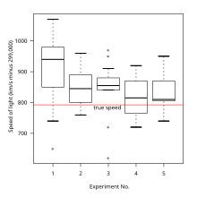
Simple L-estimators can be visually estimated from a
296:
is even, it is the average of two order statistics:
1105:
815:
667:
360:
288:
259:
219:
180:
145:
602:to make it an unbiased consistent estimator; see
926:
773:). Using two points, a simple estimate is the
741:For example, in terms of efficiency, given a
738:contain a significant amount of information.
8:
530:; many can even be computed mentally from a
407:; with a fixed fraction of the points, the
963:, Appendix G: Inefficient statistics, pp.
941:
906:Learn how and when to remove this message
806:
804:
648:
630:
619:
614:
586:, such as when using an L-estimator as a
350:
329:
310:
301:
272:
249:
232:
199:
193:
158:
137:
118:
112:
1104:Velleman, P. F.; Hoaglin, D. C. (1981).
869:This article includes a list of general
395:), and the trimmed range (including the
87:, and in modern times robust statistics
919:
1053:Selected Papers of Frederick Mosteller
960:
511:, L-estimators have been replaced by
361:{\displaystyle (x_{(k)}+x_{(k+1)})/2}
7:
598:, one generally must multiply by a
426:, and are used as estimators for a
146:{\displaystyle x_{1},\ldots ,x_{n}}
875:it lacks sufficient corresponding
445:L-estimators can also measure the
434:, and are used as estimators of a
14:
609:For example, dividing the IQR by
64:which is a linear combination of
1031:. New York: Wiley-Interscience.
977:Evans, Robley Dunglison (1955).
860:
577:Pearson's skewness coefficients
563:For example, when estimating a
656:
642:
347:
342:
330:
317:
311:
303:
246:
234:
212:
200:
1:
419:; with all points, the mean.
1088:. Berlin: Springer-Verlag.
1067:10.1007/978-0-387-44956-2_4
927:Velleman & Hoaglin 1981
816:{\displaystyle {\sqrt {n}}}
604:scale parameter: estimation
1164:
590:, such as to estimate the
442:of a normal distribution.
403:); with three points, the
188:is odd, the median equals
749:numerical parameter, the
544:non-parametric statistics
484:has a breakdown point of
391:mid-range, including the
220:{\displaystyle x_{(k+1)}}
1138:Nonparametric statistics
1027:Huber, Peter J. (2004).
588:robust measures of scale
497:robust measures of scale
267:-th order statistic; if
1086:Mathematical statistics
890:more precise citations.
723:statistically resistant
538:, or visualized from a
470:statistically resistant
468:L-estimators are often
260:{\displaystyle (n+1)/2}
99:A basic example is the
817:
704:electronic calculators
669:
524:descriptive statistics
432:statistical dispersion
362:
290:
261:
221:
182:
181:{\displaystyle n=2k+1}
147:
77:descriptive statistics
45:
818:
670:
363:
291:
262:
222:
183:
148:
19:
1047:Mosteller, Frederick
803:
747:normally-distributed
613:
558:consistent estimator
551:parameter estimation
536:seven-number summary
528:statistics education
507:In practical use in
300:
289:{\displaystyle n=2k}
271:
231:
192:
157:
111:
81:statistics education
681:normal distribution
592:population variance
532:five-number summary
397:interquartile range
26:interquartile range
1084:Shao, Jun (2003).
1020:10.1007/BF02595872
980:The Atomic Nucleus
813:
753:(average) for the
665:
596:standard deviation
582:When estimating a
573:nonparametric skew
565:location parameter
440:standard deviation
428:location parameter
413:interquartile mean
358:
286:
257:
217:
178:
143:
46:
1143:Robust statistics
1076:978-0-387-20271-6
1029:Robust statistics
916:
915:
908:
811:
793:interdecile range
624:
509:robust statistics
401:interdecile range
73:robust statistics
1155:
1123:
1111:
1099:
1080:
1056:
1042:
1023:
998:
968:
958:
945:
939:
930:
924:
911:
904:
900:
897:
891:
886:this article by
877:inline citations
864:
863:
856:
822:
820:
819:
814:
812:
807:
716:machine-readable
674:
672:
671:
666:
652:
638:
637:
625:
620:
472:, having a high
424:central tendency
367:
365:
364:
359:
354:
346:
345:
321:
320:
295:
293:
292:
287:
266:
264:
263:
258:
253:
226:
224:
223:
218:
216:
215:
187:
185:
184:
179:
152:
150:
149:
144:
142:
141:
123:
122:
66:order statistics
1163:
1162:
1158:
1157:
1156:
1154:
1153:
1152:
1128:
1127:
1126:
1120:
1103:
1096:
1083:
1077:
1045:
1039:
1026:
1001:
995:
976:
972:
971:
959:
948:
940:
933:
925:
921:
912:
901:
895:
892:
882:Please help to
881:
865:
861:
854:
837:
801:
800:
751:arithmetic mean
735:
727:breakdown point
725:, having a 50%
697:
626:
611:
610:
584:scale parameter
505:
482:Winsorized mean
474:breakdown point
466:
436:scale parameter
417:Winsorized mean
325:
306:
298:
297:
269:
268:
229:
228:
195:
190:
189:
155:
154:
133:
114:
109:
108:
97:
12:
11:
5:
1161:
1159:
1151:
1150:
1145:
1140:
1130:
1129:
1125:
1124:
1118:
1101:
1094:
1081:
1075:
1043:
1037:
1024:
1014:(2): 255–317.
999:
993:
973:
970:
969:
946:
942:Mosteller 2006
931:
918:
917:
914:
913:
868:
866:
859:
853:
850:
849:
848:
843:
836:
833:
810:
734:
731:
696:
693:
689:expected value
677:error function
664:
661:
658:
655:
651:
647:
644:
641:
636:
633:
629:
623:
618:
594:or population
504:
501:
465:
462:
438:, such as the
357:
353:
349:
344:
341:
338:
335:
332:
328:
324:
319:
316:
313:
309:
305:
285:
282:
279:
276:
256:
252:
248:
245:
242:
239:
236:
214:
211:
208:
205:
202:
198:
177:
174:
171:
168:
165:
162:
140:
136:
132:
129:
126:
121:
117:
96:
93:
24:, and include
13:
10:
9:
6:
4:
3:
2:
1160:
1149:
1146:
1144:
1141:
1139:
1136:
1135:
1133:
1121:
1119:0-87150-409-X
1115:
1110:
1109:
1102:
1097:
1095:0-387-95382-5
1091:
1087:
1082:
1078:
1072:
1068:
1064:
1060:
1055:
1054:
1048:
1044:
1040:
1038:0-471-65072-2
1034:
1030:
1025:
1021:
1017:
1013:
1009:
1005:
1000:
996:
990:
986:
982:
981:
975:
974:
966:
962:
957:
955:
953:
951:
947:
943:
938:
936:
932:
928:
923:
920:
910:
907:
899:
889:
885:
879:
878:
872:
867:
858:
857:
851:
847:
844:
842:
839:
838:
834:
832:
830:
826:
808:
797:
794:
789:
787:
783:
780:
776:
772:
768:
762:
760:
756:
752:
748:
744:
739:
732:
730:
728:
724:
719:
717:
713:
709:
705:
700:
694:
692:
690:
684:
682:
678:
662:
659:
653:
649:
645:
639:
634:
631:
627:
621:
616:
607:
605:
601:
597:
593:
589:
585:
580:
578:
574:
570:
566:
561:
559:
556:
552:
547:
545:
541:
537:
533:
529:
525:
520:
518:
514:
510:
502:
500:
498:
493:
489:
487:
483:
480:% trimmed or
479:
475:
471:
463:
461:
459:
454:
452:
448:
443:
441:
437:
433:
429:
425:
420:
418:
414:
410:
406:
402:
398:
394:
390:
386:
382:
378:
374:
369:
355:
351:
339:
336:
333:
326:
322:
314:
307:
283:
280:
277:
274:
254:
250:
243:
240:
237:
209:
206:
203:
196:
175:
172:
169:
166:
163:
160:
138:
134:
130:
127:
124:
119:
115:
106:
102:
94:
92:
90:
86:
82:
78:
74:
69:
67:
63:
59:
55:
51:
43:
39:
35:
31:
27:
23:
18:
1107:
1100:– sec. 5.2.2
1085:
1052:
1028:
1011:
1007:
994:0-89874414-8
979:
922:
902:
893:
874:
828:
824:
798:
796:efficiency.
790:
770:
763:
740:
736:
720:
701:
698:
685:
608:
600:scale factor
581:
562:
548:
521:
513:M-estimators
506:
503:Applications
494:
490:
485:
477:
467:
455:
444:
421:
409:trimmed mean
370:
104:
98:
89:M-estimators
70:
57:
53:
47:
888:introducing
846:M-estimator
759:sample mean
675:(using the
411:(including
85:inefficient
58:L-statistic
54:L-estimator
1132:Categories
961:Evans 1955
896:April 2013
871:references
852:References
755:population
733:Efficiency
712:punch card
695:Advantages
517:efficiency
464:Robustness
415:) and the
385:midsummary
50:statistics
1148:Estimator
782:mid-range
777:(the 25%
708:computers
660:≈
640:
632:−
458:L-moments
377:mid-range
128:…
62:estimator
38:mid-range
841:L-moment
835:See also
775:midhinge
555:unbiased
540:box plot
451:skewness
393:midhinge
373:quantile
103:. Given
95:Examples
60:) is an
30:midhinge
22:box plot
965:902–904
884:improve
786:trimean
779:trimmed
456:Sample
405:trimean
389:trimmed
107:values
42:trimean
1116:
1092:
1073:
1061:–100.
1035:
1004:He, X.
991:
873:, but
767:median
743:sample
383:, the
379:, the
227:, the
101:median
40:, and
745:of a
663:1.349
575:(and
447:shape
381:range
153:, if
79:, in
52:, an
34:range
1114:ISBN
1090:ISBN
1071:ISBN
1033:ISBN
1008:Test
989:ISBN
706:and
569:skew
526:and
399:and
56:(or
1063:doi
1016:doi
985:972
628:erf
534:or
488:%.
48:In
1134::
1112:.
1069:.
1059:69
1010:.
987:.
949:^
934:^
683:.
606:.
546:.
499:.
36:,
32:,
28:,
1122:.
1098:.
1079:.
1065::
1041:.
1022:.
1018::
1012:8
997:.
967:.
944:.
929:.
909:)
903:(
898:)
894:(
880:.
829:n
825:n
809:n
771:n
657:)
654:2
650:/
646:1
643:(
635:1
622:2
617:2
486:n
478:n
387:(
356:2
352:/
348:)
343:)
340:1
337:+
334:k
331:(
327:x
323:+
318:)
315:k
312:(
308:x
304:(
284:k
281:2
278:=
275:n
255:2
251:/
247:)
244:1
241:+
238:n
235:(
213:)
210:1
207:+
204:k
201:(
197:x
176:1
173:+
170:k
167:2
164:=
161:n
139:n
135:x
131:,
125:,
120:1
116:x
105:n
44:.
Text is available under the Creative Commons Attribution-ShareAlike License. Additional terms may apply.