785:, an input domain with a complex geometry is partitioned into elements with simpler shapes; for instance, two-dimensional domains (either subsets of the Euclidean plane or surfaces in three dimensions) are often partitioned into triangles. It is important for the convergence of the finite element methods that these elements be well shaped; in the case of triangles, often elements that are nearly equilateral triangles are preferred. Lloyd's algorithm can be used to smooth a mesh generated by some other algorithm, moving its vertices and changing the connection pattern among its elements in order to produce triangles that are more closely equilateral. These applications typically use a smaller number of iterations of Lloyd's algorithm, stopping it to convergence, in order to preserve other features of the mesh such as differences in element size in different parts of the mesh. In contrast to a different smoothing method,
140:
128:
116:
104:
801:. The Euclidean distance plays two roles in the algorithm: it is used to define the Voronoi cells, but it also corresponds to the choice of the centroid as the representative point of each cell, since the centroid is the point that minimizes the average squared Euclidean distance to the points in its cell. Alternative distances, and alternative central points than the centroid, may be used instead. For example,
789:(in which mesh vertices are moved to the average of their neighbors' positions), Lloyd's algorithm can change the topology of the mesh, leading to more nearly equilateral elements as well as avoiding the problems with tangling that can arise with Laplacian smoothing. However, Laplacian smoothing can be applied more generally to meshes with non-triangular elements.
813:. In this application, despite varying the metric, Hausner continued to use centroids as the representative points of their Voronoi cells. However, for metrics that differ more significantly from Euclidean, it may be appropriate to choose the minimizer of average squared distance as the representative point, in place of the centroid.
737:
The algorithm converges slowly or, due to limitations in numerical precision, may not converge. Therefore, real-world applications of Lloyd's algorithm typically stop once the distribution is "good enough." One common termination criterion is to stop when the maximum distance moved by any site in an
729:
Each time a relaxation step is performed, the points are left in a slightly more even distribution: closely spaced points move farther apart, and widely spaced points move closer together. In one dimension, this algorithm has been shown to converge to a centroidal
Voronoi diagram, also named a
182:
of point sites in the input domain. In mesh-smoothing applications, these would be the vertices of the mesh to be smoothed; in other applications they may be placed at random or by intersecting a uniform triangular mesh of the appropriate size with the input domain.
213:
Because
Voronoi diagram construction algorithms can be highly non-trivial, especially for inputs of dimension higher than two, the steps of calculating this diagram and finding the exact centroids of its cells may be replaced by an approximation.
170:. Lloyd's work became widely circulated but remained unpublished until 1982. A similar algorithm was developed independently by Joel Max and published in 1960, which is why the algorithm is sometimes referred as the Lloyd-Max algorithm.
50:
of each set in the partition and then re-partitions the input according to which of these centroids is closest. In this setting, the mean operation is an integral over a region of space, and the nearest centroid operation results in
226:
in graphics hardware. Cells are materialized as pixels, labeled with their corresponding site-ID. A cell's new center is approximated by averaging the positions of all pixels assigned with the same label. Alternatively,
719:
538:
231:
may be used, in which random sample points are generated according to some fixed underlying probability distribution, assigned to the closest site, and averaged to approximate the centroid for each site.
809:(with locally varying orientations) to find a tiling of an image by approximately square tiles whose orientation aligns with features of an image, which he used to simulate the construction of tiled
602:
421:
96:
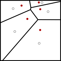
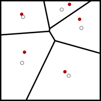
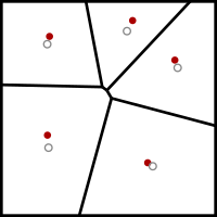
Example of Lloyd's algorithm. The
Voronoi diagram of the current site positions (red) at each iteration is shown. The gray circles denote the centroids of the Voronoi cells.
311:
754:
Lloyd's method was originally used for scalar quantization, but it is clear that the method extends for vector quantization as well. As such, it is extensively used in
629:
448:
1312:
770:), meaning there are few low-frequency components that could be interpreted as artifacts. It is particularly well-suited to picking sample positions for
1014:
866:
1081:
Deussen, Oliver; Hiller, Stefan; van
Overveld, Cornelius; Strothotte, Thomas (2000), "Floating points: a method for computing stipple drawings",
941:
641:
460:
254:
Since a
Voronoi cell is of convex shape and always encloses its site, there exist trivial decompositions into easy integratable simplices:
778:. In this application, the centroids can be weighted based on a reference image to produce stipple illustrations matching an input image.
738:
iteration falls below a preset threshold. Convergence can be accelerated by over-relaxing the points, which is done by moving each point
823:
71:
151:
In the last image, the sites are very near the centroids of the
Voronoi cells. A centroidal Voronoi tessellation has been found.
731:
67:
258:
In two dimensions, the edges of the polygonal cell are connected with its site, creating an umbrella-shaped set of triangles.
1041:
Emelianenko, Maria; Ju, Lili; Rand, Alexander (2009), "Nondegeneracy and Weak Global
Convergence of the Lloyd Algorithm in
1307:
1012:
Sabin, M. J.; Gray, R. M. (1986), "Global convergence and empirical consistency of the generalized Lloyd algorithm",
1247:; Wortman, Kevin A. (2010), "Planar Voronoi diagrams for sums of convex functions, smoothed distance and dilation",
1291:
35:
or relaxation, is an algorithm named after Stuart P. Lloyd for finding evenly spaced sets of points in subsets of
222:
A common simplification is to employ a suitable discretization of space like a fine pixel-grid, e.g. the texture
829:
284:(center of mass) is now given as a weighted combination of its simplices' centroids (in the following called
39:
and partitions of these subsets into well-shaped and uniformly sized convex cells. Like the closely related
546:
365:
1177:
1090:
984:
261:
In three dimensions, the cell is enclosed by several planar polygons which have to be triangulated first:
63:
20:
904:; Faber, Vance; Gunzburger, Max (1999), "Centroidal Voronoi tessellations: applications and algorithms",
1168:; Gunzburger, Max (2002), "Grid generation and optimization based on centroidal Voronoi tessellations",
975:; Ju, Lili (2006), "Convergence of the Lloyd algorithm for computing centroidal Voronoi tessellations",
782:
167:
87:
267:
Connecting the vertices of a polygon face with its center gives a planar umbrella-shaped triangulation.
1294:
Graphical
Javascript simulator for LBG algorithm and other models, includes display of Voronoi regions
343:
is found as the intersection of three bisector planes and can be expressed as a matrix-vector product.
1240:
913:
1182:
1095:
989:
786:
228:
1071:
Xiao, Xiao. "Over-relaxation Lloyd method for computing centroidal
Voronoi tessellations." (2010).
287:
1270:
1252:
1222:
1147:
1108:
883:
759:
251:
and discusses the two most relevant scenarios, which are two, and respectively three dimensions.
241:
40:
972:
62:, similar algorithms may also be applied to higher-dimensional spaces or to spaces with other
1262:
1249:
Proc. 7th
International Symposium on Voronoi Diagrams in Science and Engineering (ISVD 2010)
1214:
1187:
1139:
1100:
1054:
1023:
994:
950:
921:
875:
806:
755:
24:
742:
times the distance to the center of mass, typically using a value slightly less than 2 for
798:
767:
191:
59:
52:
36:
1207:
Proceedings of the 28th annual conference on Computer graphics and interactive techniques
917:
1244:
607:
426:
1191:
1301:
762:. Lloyd's method is used in computer graphics because the resulting distribution has
83:
1274:
1151:
887:
1226:
1210:
1135:
1116:
1112:
1132:
Proceedings of the Symposium on Non-Photorealistic Animation and Rendering (NPAR)
841:
632:
340:
271:
223:
925:
835:
763:
240:
Although embedding in other spaces is also possible, this elaboration assumes
1027:
954:
879:
201:
Each cell of the Voronoi diagram is integrated, and the centroid is computed.
1104:
832:, a different method for generating evenly spaced points in geometric spaces
775:
771:
734:. In higher dimensions, some slightly weaker convergence results are known.
274:
is obtained by connecting triangles of the cell's hull with the cell's site.
264:
Compute a center for the polygon face, e.g. the average of all its vertices.
163:
139:
79:
75:
66:
metrics. Lloyd's algorithm can be used to construct close approximations to
127:
115:
103:
1218:
1143:
774:. Lloyd's algorithm is also used to generate dot drawings in the style of
1266:
1165:
968:
901:
451:
321:
281:
245:
47:
714:{\displaystyle C={\frac {1}{V_{C}}}\sum _{i=0}^{n}\mathbf {c} _{i}v_{i}}
533:{\displaystyle C={\frac {1}{A_{C}}}\sum _{i=0}^{n}\mathbf {c} _{i}a_{i}}
1058:
998:
810:
1257:
178:
Lloyd's algorithm starts by an initial placement of some number
320:
For a triangle the centroid can be easily computed, e.g. using
82:. Other applications of Lloyd's algorithm include smoothing of
864:
Lloyd, Stuart P. (1982), "Least squares quantization in PCM",
826:, a generalization of this algorithm for vector quantization
204:
Each site is then moved to the centroid of its Voronoi cell.
838:, a related method for finding maxima of a density function
186:
It then repeatedly executes the following relaxation step:
58:
Although the algorithm may be applied most directly to the
1205:
Hausner, Alejo (2001), "Simulating decorative mosaics",
939:
Max, Joel (1960), "Quantizing for minimum distortion",
162:
The algorithm was first proposed by Stuart P. Lloyd of
610:
549:
429:
368:
290:
1130:
Secord, Adrian (2002), "Weighted Voronoi stippling",
644:
463:
713:
623:
596:
532:
442:
415:
305:
454:simplex), the new cell centroid computes as:
362:triangular simplices and an accumulated area
280:Integration of a cell and computation of its
8:
543:Analogously, for a 3D cell with a volume of
16:Algorithm used for points in euclidean space
1256:
1181:
1094:
988:
705:
695:
690:
683:
672:
660:
651:
643:
615:
609:
588:
578:
567:
554:
548:
524:
514:
509:
502:
491:
479:
470:
462:
434:
428:
407:
397:
386:
373:
367:
297:
292:
289:
1015:IEEE Transactions on Information Theory
867:IEEE Transactions on Information Theory
853:
802:
797:Lloyd's algorithm is usually used in a
597:{\textstyle V_{C}=\sum _{i=0}^{n}v_{i}}
416:{\textstyle A_{C}=\sum _{i=0}^{n}a_{i}}
942:IRE Transactions on Information Theory
346:Weighting computes as simplex-to-cell
327:Weighting computes as simplex-to-cell
859:
857:
7:
635:simplex), the centroid computes as:
209:Integration and centroid computation
70:of the input, which can be used for
1313:Optimization algorithms and methods
1170:Applied Mathematics and Computation
46:algorithm, it repeatedly finds the
1047:SIAM Journal on Numerical Analysis
977:SIAM Journal on Numerical Analysis
14:
691:
510:
293:
138:
126:
114:
102:
68:centroidal Voronoi tessellations
732:centroidal Voronoi tessellation
1:
1192:10.1016/S0096-3003(01)00260-0
306:{\textstyle \mathbf {c} _{i}}
166:in 1957 as a technique for
1329:
766:characteristics (see also
926:10.1137/S0036144599352836
824:Linde–Buzo–Gray algorithm
341:centroid of a tetrahedron
1028:10.1109/TIT.1986.1057168
955:10.1109/TIT.1960.1057548
880:10.1109/TIT.1982.1056489
830:Farthest-first traversal
1105:10.1111/1467-8659.00396
1083:Computer Graphics Forum
633:volume of a tetrahedron
805:used a variant of the
715:
688:
625:
598:
583:
534:
507:
444:
417:
402:
307:
21:electrical engineering
1241:Dickerson, Matthew T.
1219:10.1145/383259.383327
1144:10.1145/508530.508537
783:finite element method
716:
668:
626:
599:
563:
535:
487:
445:
418:
382:
322:cartesian coordinates
308:
174:Algorithm description
168:pulse-code modulation
88:finite element method
1308:Geometric algorithms
1267:10.1109/ISVD.2010.12
1213:, pp. 573–580,
642:
608:
547:
461:
427:
366:
288:
270:Trivially, a set of
918:1999SIAMR..41..637D
793:Different distances
787:Laplacian smoothing
356:For a 2D cell with
229:Monte Carlo methods
1251:, pp. 13–22,
1138:, pp. 37–43,
973:Emelianenko, Maria
760:information theory
711:
624:{\textstyle v_{i}}
621:
594:
530:
452:area of a triangle
443:{\textstyle a_{i}}
440:
413:
336:Three dimensions:
303:
198:sites is computed.
1115:, Proceedings of
1059:10.1137/070691334
999:10.1137/040617364
666:
485:
236:Exact computation
44:-means clustering
33:Voronoi iteration
29:Lloyd's algorithm
1320:
1279:
1277:
1260:
1237:
1231:
1229:
1202:
1196:
1194:
1185:
1176:(2–3): 591–607,
1162:
1156:
1154:
1127:
1121:
1119:
1098:
1078:
1072:
1069:
1063:
1061:
1038:
1032:
1030:
1009:
1003:
1001:
992:
965:
959:
957:
936:
930:
928:
898:
892:
890:
861:
807:Manhattan metric
756:data compression
720:
718:
717:
712:
710:
709:
700:
699:
694:
687:
682:
667:
665:
664:
652:
630:
628:
627:
622:
620:
619:
603:
601:
600:
595:
593:
592:
582:
577:
559:
558:
539:
537:
536:
531:
529:
528:
519:
518:
513:
506:
501:
486:
484:
483:
471:
449:
447:
446:
441:
439:
438:
422:
420:
419:
414:
412:
411:
401:
396:
378:
377:
361:
317:Two dimensions:
312:
310:
309:
304:
302:
301:
296:
142:
130:
118:
106:
53:Voronoi diagrams
37:Euclidean spaces
31:, also known as
25:computer science
1328:
1327:
1323:
1322:
1321:
1319:
1318:
1317:
1298:
1297:
1288:
1283:
1282:
1245:Eppstein, David
1239:
1238:
1234:
1204:
1203:
1199:
1183:10.1.1.324.5020
1164:
1163:
1159:
1129:
1128:
1124:
1096:10.1.1.233.5810
1080:
1079:
1075:
1070:
1066:
1040:
1039:
1035:
1011:
1010:
1006:
990:10.1.1.591.9903
967:
966:
962:
938:
937:
933:
900:
899:
895:
863:
862:
855:
850:
819:
799:Euclidean space
795:
768:Colors of noise
752:
727:
701:
689:
656:
640:
639:
611:
606:
605:
584:
550:
545:
544:
520:
508:
475:
459:
458:
430:
425:
424:
403:
369:
364:
363:
357:
291:
286:
285:
242:Euclidean space
238:
220:
211:
192:Voronoi diagram
176:
160:
155:
154:
153:
152:
148:
147:
146:
143:
135:
134:
131:
123:
122:
119:
111:
110:
107:
98:
97:
84:triangle meshes
60:Euclidean plane
17:
12:
11:
5:
1326:
1324:
1316:
1315:
1310:
1300:
1299:
1296:
1295:
1287:
1286:External links
1284:
1281:
1280:
1232:
1197:
1157:
1122:
1073:
1064:
1033:
1022:(2): 148–155,
1004:
960:
931:
912:(4): 637–676,
893:
874:(2): 129–137,
852:
851:
849:
846:
845:
844:
839:
833:
827:
818:
815:
803:Hausner (2001)
794:
791:
758:techniques in
751:
748:
726:
723:
722:
721:
708:
704:
698:
693:
686:
681:
678:
675:
671:
663:
659:
655:
650:
647:
618:
614:
591:
587:
581:
576:
573:
570:
566:
562:
557:
553:
541:
540:
527:
523:
517:
512:
505:
500:
497:
494:
490:
482:
478:
474:
469:
466:
437:
433:
410:
406:
400:
395:
392:
389:
385:
381:
376:
372:
354:
353:
352:
351:
344:
334:
333:
332:
325:
300:
295:
278:
277:
276:
275:
268:
265:
259:
237:
234:
219:
216:
210:
207:
206:
205:
202:
199:
175:
172:
159:
156:
150:
149:
144:
137:
136:
132:
125:
124:
120:
113:
112:
108:
101:
100:
99:
95:
94:
93:
92:
15:
13:
10:
9:
6:
4:
3:
2:
1325:
1314:
1311:
1309:
1306:
1305:
1303:
1293:
1290:
1289:
1285:
1276:
1272:
1268:
1264:
1259:
1254:
1250:
1246:
1242:
1236:
1233:
1228:
1224:
1220:
1216:
1212:
1208:
1201:
1198:
1193:
1189:
1184:
1179:
1175:
1171:
1167:
1161:
1158:
1153:
1149:
1145:
1141:
1137:
1133:
1126:
1123:
1118:
1114:
1110:
1106:
1102:
1097:
1092:
1088:
1084:
1077:
1074:
1068:
1065:
1060:
1056:
1053:: 1423–1441,
1052:
1048:
1044:
1037:
1034:
1029:
1025:
1021:
1017:
1016:
1008:
1005:
1000:
996:
991:
986:
982:
978:
974:
970:
964:
961:
956:
952:
948:
944:
943:
935:
932:
927:
923:
919:
915:
911:
907:
903:
897:
894:
889:
885:
881:
877:
873:
869:
868:
860:
858:
854:
847:
843:
840:
837:
834:
831:
828:
825:
821:
820:
816:
814:
812:
808:
804:
800:
792:
790:
788:
784:
779:
777:
773:
769:
765:
761:
757:
749:
747:
745:
741:
735:
733:
724:
706:
702:
696:
684:
679:
676:
673:
669:
661:
657:
653:
648:
645:
638:
637:
636:
634:
616:
612:
589:
585:
579:
574:
571:
568:
564:
560:
555:
551:
525:
521:
515:
503:
498:
495:
492:
488:
480:
476:
472:
467:
464:
457:
456:
455:
453:
435:
431:
408:
404:
398:
393:
390:
387:
383:
379:
374:
370:
360:
349:
345:
342:
338:
337:
335:
330:
326:
323:
319:
318:
316:
315:
314:
298:
283:
273:
269:
266:
263:
262:
260:
257:
256:
255:
252:
250:
248:
243:
235:
233:
230:
225:
218:Approximation
217:
215:
208:
203:
200:
197:
193:
189:
188:
187:
184:
181:
173:
171:
169:
165:
157:
141:
129:
117:
105:
91:
89:
85:
81:
77:
73:
69:
65:
64:non-Euclidean
61:
56:
54:
49:
45:
43:
38:
34:
30:
26:
22:
1248:
1235:
1211:ACM SIGGRAPH
1206:
1200:
1173:
1169:
1160:
1136:ACM SIGGRAPH
1131:
1125:
1117:Eurographics
1089:(3): 41–50,
1086:
1082:
1076:
1067:
1050:
1046:
1042:
1036:
1019:
1013:
1007:
980:
976:
963:
946:
940:
934:
909:
905:
896:
871:
865:
796:
780:
753:
750:Applications
743:
739:
736:
728:
542:
358:
355:
347:
328:
279:
253:
246:
239:
221:
212:
195:
185:
179:
177:
161:
145:Iteration 15
72:quantization
57:
41:
32:
28:
18:
983:: 102–119,
949:(1): 7–12,
906:SIAM Review
725:Convergence
133:Iteration 3
121:Iteration 2
109:Iteration 1
1302:Categories
1292:DemoGNG.js
848:References
836:Mean shift
764:blue noise
272:tetrahedra
244:using the
1258:0812.0607
1178:CiteSeerX
1166:Du, Qiang
1091:CiteSeerX
985:CiteSeerX
969:Du, Qiang
902:Du, Qiang
842:K-means++
776:stippling
772:dithering
670:∑
565:∑
489:∑
384:∑
164:Bell Labs
80:stippling
76:dithering
1275:15971504
1152:12153589
888:10833328
817:See also
282:centroid
48:centroid
1227:7188986
914:Bibcode
811:mosaics
781:In the
631:is the
604:(where
450:is the
423:(where
350:ratios.
331:ratios.
194:of the
158:History
86:in the
1273:
1225:
1180:
1150:
1113:142991
1111:
1093:
987:
886:
348:volume
224:buffer
78:, and
1271:S2CID
1253:arXiv
1223:S2CID
1148:S2CID
1109:S2CID
884:S2CID
822:The
339:The
329:area
249:norm
190:The
23:and
1263:doi
1215:doi
1188:doi
1174:133
1140:doi
1101:doi
1055:doi
1045:",
1024:doi
995:doi
951:doi
922:doi
876:doi
313:).
19:In
1304::
1269:,
1261:,
1243:;
1221:,
1209:,
1186:,
1172:,
1146:,
1134:,
1107:,
1099:,
1087:19
1085:,
1051:46
1049:,
1020:32
1018:,
993:,
981:44
979:,
971:;
945:,
920:,
910:41
908:,
882:,
872:28
870:,
856:^
746:.
90:.
74:,
55:.
27:,
1278:.
1265::
1255::
1230:.
1217::
1195:.
1190::
1155:.
1142::
1120:.
1103::
1062:.
1057::
1043:R
1031:.
1026::
1002:.
997::
958:.
953::
947:6
929:.
924::
916::
891:.
878::
744:ω
740:ω
707:i
703:v
697:i
692:c
685:n
680:0
677:=
674:i
662:C
658:V
654:1
649:=
646:C
617:i
613:v
590:i
586:v
580:n
575:0
572:=
569:i
561:=
556:C
552:V
526:i
522:a
516:i
511:c
504:n
499:0
496:=
493:i
481:C
477:A
473:1
468:=
465:C
436:i
432:a
409:i
405:a
399:n
394:0
391:=
388:i
380:=
375:C
371:A
359:n
324:.
299:i
294:c
247:L
196:k
180:k
42:k
Text is available under the Creative Commons Attribution-ShareAlike License. Additional terms may apply.