4236:
279:(CDF), all quantiles are uniquely defined and can be obtained by inverting the CDF. If a theoretical probability distribution with a discontinuous CDF is one of the two distributions being compared, some of the quantiles may not be defined, so an interpolated quantile may be plotted. If the Q–Q plot is based on data, there are multiple quantile estimators in use. Rules for forming Q–Q plots when quantiles must be estimated or interpolated are called
40:
4222:
78:
99:
257:
4260:
87:
4248:
1801:
421:
Although a Q–Q plot is based on quantiles, in a standard Q–Q plot it is not possible to determine which point in the Q–Q plot determines a given quantile. For example, it is not possible to determine the median of either of the two distributions being compared by inspecting the Q–Q plot. Some Q–Q
286:
A simple case is where one has two data sets of the same size. In that case, to make the Q–Q plot, one orders each set in increasing order, then pairs off and plots the corresponding values. A more complicated construction is the case where two data sets of different sizes are being compared. To
425:
The intercept and slope of a linear regression between the quantiles gives a measure of the relative location and relative scale of the samples. If the median of the distribution plotted on the horizontal axis is 0, the intercept of a regression line is a measure of location, and the slope is a
434:
between the paired sample quantiles. The closer the correlation coefficient is to one, the closer the distributions are to being shifted, scaled versions of each other. For distributions with a single shape parameter, the probability plot correlation coefficient plot provides a method for
1221:
563:
Many other choices have been suggested, both formal and heuristic, based on theory or simulations relevant in context. The following subsections discuss some of these. A narrower question is choosing a maximum (estimation of a population maximum), known as the
685:
This can be easily generated for any distribution for which the quantile function can be computed, but conversely the resulting estimates of location and scale are no longer precisely the least squares estimates, though these only differ significantly for
417:
than the distribution plotted on the horizontal axis. Q–Q plots are often arced, or S-shaped, indicating that one of the distributions is more skewed than the other, or that one of the distributions has heavier tails than the other.
435:
estimating the shape parameter – one simply computes the correlation coefficient for different values of the shape parameter, and uses the one with the best fit, just as if one were comparing distributions of different types.
1805:
81:
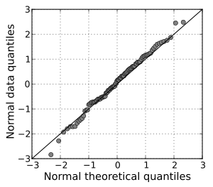
A normal Q–Q plot comparing randomly generated, independent standard normal data on the vertical axis to a standard normal population on the horizontal axis. The linearity of the points suggests that the data are normally
660:
of the fitted line). Although this is not too important for the normal distribution (the location and scale are estimated by the mean and standard deviation, respectively), it can be useful for many other distributions.
1035:
248:(PPCC plot) is a quantity derived from the idea of Q–Q plots, which measures the agreement of a fitted distribution with observed data and which is sometimes used as a means of fitting a distribution to data.
678:
of the order statistics, which one can compute based on estimates of the median of the order statistics of a uniform distribution and the quantile function of the distribution; this was suggested by
275:
The main step in constructing a Q–Q plot is calculating or estimating the quantiles to be plotted. If one or both of the axes in a Q–Q plot is based on a theoretical distribution with a continuous
452:. As in the case when comparing two samples of data, one orders the data (formally, computes the order statistics), then plots them against certain quantiles of the theoretical distribution.
272:
is a plot of the quantiles of two distributions against each other, or a plot based on estimates of the quantiles. The pattern of points in the plot is used to compare the two distributions.
233:. Q–Q plots are also used to compare two theoretical distributions to each other. Since Q–Q plots compare distributions, there is no need for the values to be observed as pairs, as in a
369:
The points plotted in a Q–Q plot are always non-decreasing when viewed from left to right. If the two distributions being compared are identical, the Q–Q plot follows the 45° line
994:
379:. If the two distributions agree after linearly transforming the values in one of the distributions, then the Q–Q plot follows some line, but not necessarily the line
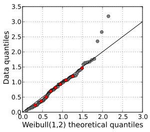
94:. The deciles of the distributions are shown in red. Three outliers are evident at the high end of the range. Otherwise, the data fit the Weibull(1,2) model well.
3357:
431:
3862:
245:
547:
240:
The term "probability plot" sometimes refers specifically to a Q–Q plot, sometimes to a more general class of plots, and sometimes to the less commonly used
4012:
3636:
2277:
500:, corresponds to the 100th percentile – the maximum value of the theoretical distribution, which is sometimes infinite. Other choices are the use of
73:). The offset between the line and the points suggests that the mean of the data is not 0. The median of the points can be determined to be near 0.7
4286:
3410:
427:
3849:
1026:
is less than or equal to some value). That is, given a probability, we want the corresponding quantile of the cumulative distribution function.
1216:{\displaystyle m(i)={\begin{cases}1-0.5^{1/n}&i=1\\\\{\dfrac {i-0.3175}{n+0.365}}&i=2,3,\ldots ,n-1\\\\0.5^{1/n}&i=n.\end{cases}}}
1890:
1769:
1688:
1597:
66:
on the horizontal axis. The points follow a strongly nonlinear pattern, suggesting that the data are not distributed as a standard normal (
2272:
1972:
184:. If the distributions are linearly related, the points in the Q–Q plot will approximately lie on a line, but not necessarily on the line
664:
However, this requires calculating the expected values of the order statistic, which may be difficult if the distribution is not normal.
225:, but is less widely known. Q–Q plots are commonly used to compare a data set to a theoretical model. This can provide an assessment of
2876:
2024:
106:
daily maximum temperatures at 25 stations in the US state of Ohio in March and in July. The curved pattern suggests that the central
3659:
3551:
1929:
1908:
1841:
4264:
3837:
3711:
1017:
276:
460:
The choice of quantiles from a theoretical distribution can depend upon context and purpose. One choice, given a sample of size
3895:
3556:
3301:
2672:
2262:
1255:
517:
points such that there is an equal distance between all of them and also between the two outermost points and the edges of the
438:
Another common use of Q–Q plots is to compare the distribution of a sample to a theoretical distribution, such as the standard
403:
than the distribution plotted on the vertical axis. Conversely, if the general trend of the Q–Q plot is steeper than the line
2886:
3946:
3158:
2965:
2854:
2812:
2051:
221:
approach to comparing their underlying distributions. A Q–Q plot is generally more diagnostic than comparing the samples'
4189:
3148:
3198:
3740:
3689:
3674:
3664:
3533:
3405:
3372:
3153:
2983:
3809:
3110:
4084:
3885:
2864:
2533:
1997:
426:
measure of scale. The distance between medians is another measure of relative location reflected in a Q–Q plot. The "
3969:
3936:
3941:
3684:
3443:
3349:
3329:
3237:
2948:
2766:
2249:
2121:
648:
uses the expected values of the order statistics of the given distribution; the resulting plot and line yields the
584:
3115:
2881:
2739:
3701:
3469:
3190:
3044:
2973:
2893:
2751:
2732:
2440:
2161:
1285:
649:
261:
218:
127:
3814:
201:
A Q–Q plot is used to compare the shapes of distributions, providing a graphical view of how properties such as
4184:
3951:
3499:
3464:
3428:
3213:
2655:
2564:
2523:
2435:
2126:
1965:
1235:
131:
44:
3221:
3205:
171:
If the two distributions being compared are similar, the points in the Q–Q plot will approximately lie on the
213:
are similar or different in the two distributions. Q–Q plots can be used to compare collections of data, or
4093:
3706:
3646:
3583:
2943:
2805:
2795:
2645:
2559:
634:
449:
3854:
3791:
4131:
4061:
3546:
3433:
2430:
2327:
2234:
2113:
2012:
1703:
1498:
414:
400:
214:
206:
63:
4252:
3130:
645:
291:
quantile estimate so that quantiles corresponding to the same underlying probability can be constructed.
4156:
4098:
4041:
3867:
3760:
3669:
3395:
3279:
3138:
3020:
3012:
2827:
2723:
2701:
2660:
2625:
2592:
2538:
2513:
2468:
2407:
2367:
2169:
1992:
1486:
701:
487:
195:
4235:
3125:
1749:
Hazen, Allen (1914), "Storage to be provided in the impounding reservoirs for municipal water supply",
1468:
4079:
3654:
3603:
3579:
3541:
3459:
3438:
3390:
3269:
3247:
3216:
3002:
2953:
2871:
2844:
2800:
2756:
2518:
2294:
2174:
1715:
1644:
1264:
91:
1945:
1847:
Filliben, J. J. (February 1975), "The
Probability Plot Correlation Coefficient Test for Normality",
1059:
4226:
4151:
4074:
3755:
3519:
3512:
3474:
3382:
3362:
3334:
3067:
2933:
2928:
2918:
2910:
2728:
2689:
2579:
2569:
2478:
2257:
2213:
2131:
2056:
1958:
1348:
1016:
is the quantile function for the desired distribution. The quantile function is the inverse of the
565:
439:
352:
55:
3801:
946:
4240:
4051:
3905:
3750:
3626:
3523:
3507:
3484:
3261:
2995:
2978:
2938:
2849:
2744:
2706:
2677:
2637:
2597:
2543:
2460:
2146:
2141:
1864:
1570:
1424:
641:, the quantile of the expected value of the order statistic of a standard normal distribution.
4146:
4116:
4108:
3928:
3919:
3844:
3775:
3631:
3616:
3591:
3479:
3420:
3286:
3274:
2900:
2817:
2761:
2684:
2528:
2450:
2229:
2103:
1925:
1904:
1886:
1837:
1731:
1593:
1432:
1407:
Wilk, M.B.; Gnanadesikan, R. (1968), "Probability plotting methods for the analysis of data",
1365:
307:
230:
1601:
4171:
4126:
3890:
3877:
3770:
3745:
3679:
3611:
3489:
3097:
2990:
2923:
2836:
2783:
2602:
2473:
2267:
2066:
2033:
1856:
1723:
1668:
1626:
1562:
1416:
1226:
The reason for this estimate is that the order statistic medians do not have a simple form.
937:
933:
202:
606:
approach equals that of plotting the points according to the probability that the last of (
4088:
3832:
3694:
3621:
3296:
3170:
3143:
3120:
3089:
2716:
2711:
2665:
2395:
2046:
1876:
226:
165:
1719:
1347:
This plotting position was used by Irving I. Gringorten to plot points in tests for the
1029:
James J. Filliben uses the following estimates for the uniform order statistic medians:
4037:
4032:
2495:
2425:
2071:
1630:
103:
936:
of the distribution. These can be expressed in terms of the quantile function and the
520:
39:
4280:
4194:
4161:
4024:
3985:
3796:
3765:
3229:
3183:
2788:
2490:
2317:
2081:
2076:
1574:
288:
172:
114:
to the left compared to the March distribution. The data cover the period 1893–2001.
241:
31:
4136:
4069:
4046:
3961:
3291:
2587:
2485:
2420:
2362:
2284:
2239:
321:(the inverse function of the CDF is the quantile function), the Q–Q plot draws the
234:
237:, or even for the numbers of values in the two groups being compared to be equal.
1919:
1880:
1589:
1284:
Note that this also uses a different expression for the first & last points.
194:. Q–Q plots can also be used as a graphical means of estimating parameters in a
110:
are more closely spaced in July than in March, and that the July distribution is
4179:
4141:
3824:
3725:
3587:
3400:
3367:
2859:
2776:
2771:
2415:
2372:
2352:
2332:
2322:
2091:
1524:
Weibull, Waloddi (1939), "The
Statistical Theory of the Strength of Materials",
704:
653:
264:, versus a normal distribution. Outliers are visible in the upper right corner.
77:
3025:
2505:
2205:
2136:
2086:
2061:
1981:
1566:
1553:
Makkonen, L. (2008), "Bringing closure to the plotting position controversy",
568:, for which similar "sample maximum, plus a gap" solutions exist, most simply
1735:
3178:
3030:
2650:
2445:
2357:
2342:
2337:
2302:
1727:
1420:
256:
222:
152:
on the plot corresponds to one of the quantiles of the second distribution (
98:
1436:
1238:
comes with functions to make Q–Q plots, namely qqnorm and qqplot from the
217:. The use of Q–Q plots to compare two samples of data can be viewed as a
158:-coordinate) plotted against the same quantile of the first distribution (
27:
Plot of the empirical distribution of p-values against the theoretical one
2694:
2312:
2189:
2184:
2179:
2151:
422:
plots indicate the deciles to make determinations such as this possible.
294:
More abstractly, given two cumulative probability distribution functions
210:
136:
111:
107:
1317:
A simple (and easy to remember) formula for plotting positions; used in
629:
Expected value of the order statistic for a standard normal distribution
583:. A more formal application of this uniformization of spacing occurs in
4199:
3900:
1868:
1824:
Chambers, John; Cleveland, William; Kleiner, Beat; Tukey, Paul (1983),
1428:
1335:
86:
17:
4121:
3102:
3076:
3056:
2307:
2098:
1292:
1260:
674:
638:
1860:
1246:
package implements faster plotting for large number of data points.
657:
255:
97:
85:
76:
38:
389:. If the general trend of the Q–Q plot is flatter than the line
2041:
1318:
924:, there is little difference between these various expressions.
591:
Expected value of the order statistic for a uniform distribution
59:
4010:
3577:
3324:
2623:
2393:
2010:
1954:
938:
order statistic medians for the continuous uniform distribution
287:
construct the Q–Q plot in this case, it is necessary to use an
1499:"SR 20 – North Cascades Highway – Opening and Closing History"
43:
A normal Q–Q plot of randomly generated, independent standard
1950:
1901:
Methods for
Statistical Analysis of Multivariate Observations
1614:
1526:
IVA Handlingar, Royal
Swedish Academy of Engineering Sciences
1505:. Washington State Department of Transportation. October 2009
1209:
168:
where the parameter is the index of the quantile interval.
399:, the distribution plotted on the horizontal axis is more
700:
Several different formulas have been used or proposed as
413:, the distribution plotted on the vertical axis is more
1809:
1751:
Transactions of the
American Society of Civil Engineers
1334:'s earlier approximation and is the expression used in
229:
that is graphical, rather than reducing to a numerical
736:
in the range from 0 to 1, which gives a range between
1105:
1038:
949:
523:
3863:
Autoregressive conditional heteroskedasticity (ARCH)
1817:
Statistical estimates and transformed beta variables
1768:
sfnp error: no target: CITEREFLarsenCurranHunt1980 (
4170:
4107:
4060:
4023:
3978:
3960:
3927:
3918:
3876:
3823:
3784:
3733:
3724:
3645:
3602:
3532:
3498:
3452:
3419:
3381:
3348:
3260:
3169:
3088:
3043:
3011:
2964:
2909:
2835:
2826:
2636:
2578:
2552:
2504:
2459:
2406:
2293:
2248:
2222:
2204:
2160:
2112:
2032:
2023:
1615:"The plotting of observations on probability paper"
1613:Benard, A.; Bos-Levenbach, E. C. (September 1953).
1243:
1239:
932:The order statistic medians are the medians of the
1482:
1215:
988:
541:
260:Q–Q plot for first opening/final closing dates of
1555:Communications in Statistics – Theory and Methods
1763:
3411:Multivariate adaptive regression splines (MARS)
1704:"A plotting rule for extreme probability paper"
1810:National Institute of Standards and Technology
1966:
246:probability plot correlation coefficient plot
8:
1855:(1), American Society for Quality: 111–117,
1449:
1010:are the uniform order statistic medians and
672:Alternatively, one may use estimates of the
613:) randomly drawn values will not exceed the
355:indexed over with values in the real plane
1687:sfnp error: no target: CITEREFCunnane1978 (
4020:
4007:
3924:
3730:
3599:
3574:
3345:
3321:
3049:
2832:
2633:
2620:
2403:
2390:
2029:
2020:
2007:
1973:
1959:
1951:
1467:, Section 2.2.2, Quantile-Quantile Plots,
652:estimate for location and scale (from the
102:A Q–Q plot comparing the distributions of
1585:
1583:
1478:
1476:
1460:
1458:
1364:, these plotting points are equal to the
1182:
1178:
1104:
1076:
1072:
1054:
1037:
948:
522:
1782:
1361:
1291:. This expression is an estimate of the
1288:
679:
428:probability plot correlation coefficient
90:A Q–Q plot of a sample of data versus a
1682:
1399:
1277:
280:
3937:Kaplan–Meier estimator (product limit)
1592:, by Henry C. Thode, CRC Press, 2002,
486:, as these are the quantiles that the
1464:
7:
4247:
3947:Accelerated failure time (AFT) model
1331:
4259:
3542:Analysis of variance (ANOVA, anova)
1882:Nonparametric statistical inference
1826:Graphical methods for data analysis
1670:Distribution free plotting position
1645:"1.3.3.21. Normal Probability Plot"
3637:Cochran–Mantel–Haenszel statistics
2263:Pearson product-moment correlation
1879:; Chakraborti, Subhabrata (2003),
1631:10.1111/j.1467-9574.1953.tb00821.x
1539:Madsen, H.O.; et al. (1986),
25:
637:, the quantiles one uses are the
4258:
4246:
4234:
4221:
4220:
1804: This article incorporates
1799:
1764:Larsen, Curran & Hunt (1980)
1483:Gibbons & Chakraborti (2003)
1018:cumulative distribution function
277:cumulative distribution function
4287:Statistical charts and diagrams
3896:Least-squares spectral analysis
1819:, New York: John Wiley and Sons
1708:Journal of Geophysical Research
1256:Empirical distribution function
2877:Mean-unbiased minimum-variance
1702:Gringorten, Irving I. (1963).
1048:
1042:
983:
980:
974:
968:
959:
953:
710:. Such formulas have the form
668:Median of the order statistics
536:
524:
1:
4190:Geographic information system
3406:Simultaneous equations models
1834:The Elements of Graphing Data
1415:(1), Biometrika Trust: 1–17,
490:realizes. The last of these,
164:-coordinate). This defines a
54:). This Q–Q plot compares a
3373:Coefficient of determination
2984:Uniformly most powerful test
1541:Methods of Structural Safety
989:{\displaystyle N(i)=G(U(i))}
140:against each other. A point
3942:Proportional hazards models
3886:Spectral density estimation
3868:Vector autoregression (VAR)
3302:Maximum posterior estimator
2534:Randomized controlled trial
1924:, New York: Marcel Dekker,
1885:(4th ed.), CRC Press,
1287:cites the original work by
351:. Thus, the Q–Q plot is a
252:Definition and construction
126:) is a probability plot, a
4303:
3702:Multivariate distributions
2122:Average absolute deviation
1263:analysis was developed by
619:-th smallest of the first
585:maximum spacing estimation
511:, or instead to space the
62:on the vertical axis to a
29:
4216:
4019:
4006:
3690:Structural equation model
3598:
3573:
3344:
3320:
3052:
3026:Score/Lagrange multiplier
2632:
2619:
2441:Sample size determination
2402:
2389:
2019:
2006:
1988:
1899:Gnanadesikan, R. (1977).
1567:10.1080/03610920701653094
650:generalized least squares
345:for a range of values of
262:Washington State Route 20
215:theoretical distributions
132:probability distributions
4185:Environmental statistics
3707:Elliptical distributions
3500:Generalized linear model
3429:Simple linear regression
3199:Hodges–Lehmann estimator
2656:Probability distribution
2565:Stochastic approximation
2127:Coefficient of variation
1918:Thode, Henry C. (2002),
927:
30:Not to be confused with
3845:Cross-correlation (XCF)
3453:Non-standard predictors
2887:Lehmann–Scheffé theorem
2560:Adaptive clinical trial
1877:Gibbons, Jean Dickinson
1832:Cleveland, W.S. (1994)
1728:10.1029/JZ068i003p00813
918:For large sample size,
635:normal probability plot
625:randomly drawn values.
450:normal probability plot
432:correlation coefficient
4241:Mathematics portal
4062:Engineering statistics
3970:Nelson–Aalen estimator
3547:Analysis of covariance
3434:Ordinary least squares
3358:Pearson product-moment
2762:Statistical functional
2673:Empirical distribution
2506:Controlled experiments
2235:Frequency distribution
2013:Descriptive statistics
1806:public domain material
1619:Statistica Neerlandica
1236:R programming language
1217:
990:
543:
265:
124:quantile–quantile plot
115:
95:
83:
74:
64:statistical population
4157:Population statistics
4099:System identification
3833:Autocorrelation (ACF)
3761:Exponential smoothing
3675:Discriminant analysis
3670:Canonical correlation
3534:Partition of variance
3396:Regression validation
3240:(Jonckheere–Terpstra)
3139:Likelihood-ratio test
2828:Frequentist inference
2740:Location–scale family
2661:Sampling distribution
2626:Statistical inference
2593:Cross-sectional study
2580:Observational studies
2539:Randomized experiment
2368:Stem-and-leaf display
2170:Central limit theorem
1921:Testing for normality
1590:Testing for Normality
1503:North Cascades Passes
1421:10.1093/biomet/55.1.1
1218:
991:
762:Expressions include:
544:
488:sampling distribution
430:" (PPCC plot) is the
259:
196:location-scale family
101:
89:
80:
42:
4080:Probabilistic design
3665:Principal components
3508:Exponential families
3460:Nonlinear regression
3439:General linear model
3401:Mixed effects models
3391:Errors and residuals
3368:Confounding variable
3270:Bayesian probability
3248:Van der Waerden test
3238:Ordered alternative
3003:Multiple comparisons
2882:Rao–Blackwellization
2845:Estimating equations
2801:Statistical distance
2519:Factorial experiment
2052:Arithmetic-Geometric
1321:statistical package.
1265:Chester Ittner Bliss
1036:
947:
521:
92:Weibull distribution
4152:Official statistics
4075:Methods engineering
3756:Seasonal adjustment
3524:Poisson regressions
3444:Bayesian regression
3383:Regression analysis
3363:Partial correlation
3335:Regression analysis
2934:Prediction interval
2929:Likelihood interval
2919:Confidence interval
2911:Interval estimation
2872:Unbiased estimators
2690:Model specification
2570:Up-and-down designs
2258:Partial correlation
2214:Index of dispersion
2132:Interquartile range
1720:1963JGR....68..813G
1450:Gnanadesikan (1977)
1349:Gumbel distribution
928:Filliben's estimate
566:German tank problem
440:normal distribution
4172:Spatial statistics
4052:Medical statistics
3952:First hitting time
3906:Whittle likelihood
3557:Degrees of freedom
3552:Multivariate ANOVA
3485:Heteroscedasticity
3297:Bayesian estimator
3262:Bayesian inference
3111:Kolmogorov–Smirnov
2996:Randomization test
2966:Testing hypotheses
2939:Tolerance interval
2850:Maximum likelihood
2745:Exponential family
2678:Density estimation
2638:Statistical theory
2598:Natural experiment
2544:Scientific control
2461:Survey methodology
2147:Standard deviation
1213:
1208:
1130:
1020:(probability that
986:
730:for some value of
708:plotting positions
539:
456:Plotting positions
308:quantile functions
306:, with associated
281:plotting positions
266:
198:of distributions.
134:by plotting their
130:for comparing two
116:
96:
84:
75:
4274:
4273:
4212:
4211:
4208:
4207:
4147:National accounts
4117:Actuarial science
4109:Social statistics
4002:
4001:
3998:
3997:
3994:
3993:
3929:Survival function
3914:
3913:
3776:Granger causality
3617:Contingency table
3592:Survival analysis
3569:
3568:
3565:
3564:
3421:Linear regression
3316:
3315:
3312:
3311:
3287:Credible interval
3256:
3255:
3039:
3038:
2855:Method of moments
2724:Parametric family
2685:Statistical model
2615:
2614:
2611:
2610:
2529:Random assignment
2451:Statistical power
2385:
2384:
2381:
2380:
2230:Contingency table
2200:
2199:
2067:Generalized/power
1892:978-0-8247-4052-8
1815:Blom, G. (1958),
1598:978-0-8247-9613-6
1129:
646:Shapiro–Wilk test
231:summary statistic
118:In statistics, a
16:(Redirected from
4294:
4262:
4261:
4250:
4249:
4239:
4238:
4224:
4223:
4127:Crime statistics
4021:
4008:
3925:
3891:Fourier analysis
3878:Frequency domain
3858:
3805:
3771:Structural break
3731:
3680:Cluster analysis
3627:Log-linear model
3600:
3575:
3516:
3490:Homoscedasticity
3346:
3322:
3241:
3233:
3225:
3224:(Kruskal–Wallis)
3209:
3194:
3149:Cross validation
3134:
3116:Anderson–Darling
3063:
3050:
3021:Likelihood-ratio
3013:Parametric tests
2991:Permutation test
2974:1- & 2-tails
2865:Minimum distance
2837:Point estimation
2833:
2784:Optimal decision
2735:
2634:
2621:
2603:Quasi-experiment
2553:Adaptive designs
2404:
2391:
2268:Rank correlation
2030:
2021:
2008:
1975:
1968:
1961:
1952:
1946:Probability plot
1934:
1914:
1895:
1872:
1829:
1820:
1803:
1802:
1786:
1780:
1774:
1773:
1761:
1755:
1754:
1746:
1740:
1739:
1699:
1693:
1692:
1680:
1674:
1672:, Yu & Huang
1666:
1660:
1659:
1657:
1655:
1641:
1635:
1634:
1610:
1604:
1587:
1578:
1577:
1550:
1544:
1543:
1536:
1530:
1529:
1521:
1515:
1514:
1512:
1510:
1495:
1489:
1480:
1471:
1462:
1453:
1447:
1441:
1440:
1404:
1382:
1380:
1358:
1352:
1345:
1339:
1328:
1322:
1315:
1309:
1307:
1282:
1245:
1241:
1222:
1220:
1219:
1214:
1212:
1211:
1191:
1190:
1186:
1170:
1131:
1128:
1117:
1106:
1100:
1085:
1084:
1080:
1025:
1015:
1009:
995:
993:
992:
987:
934:order statistics
923:
913:
899:
885:
872:
858:
844:
830:
816:
802:
788:
775:
758:
746:
735:
729:
691:
644:More generally,
624:
618:
612:
605:
582:
559:
549:interval, using
548:
546:
545:
542:{\displaystyle }
540:
516:
510:
499:
485:
475:
465:
447:
412:
398:
388:
378:
360:
353:parametric curve
350:
344:
339:-th quantile of
338:
332:
327:-th quantile of
326:
320:
314:
305:
299:
193:
183:
166:parametric curve
163:
157:
151:
128:graphical method
72:
53:
21:
4302:
4301:
4297:
4296:
4295:
4293:
4292:
4291:
4277:
4276:
4275:
4270:
4233:
4204:
4166:
4103:
4089:quality control
4056:
4038:Clinical trials
4015:
3990:
3974:
3962:Hazard function
3956:
3910:
3872:
3856:
3819:
3815:Breusch–Godfrey
3803:
3780:
3720:
3695:Factor analysis
3641:
3622:Graphical model
3594:
3561:
3528:
3514:
3494:
3448:
3415:
3377:
3340:
3339:
3308:
3252:
3239:
3231:
3223:
3207:
3192:
3171:Rank statistics
3165:
3144:Model selection
3132:
3090:Goodness of fit
3084:
3061:
3035:
3007:
2960:
2905:
2894:Median unbiased
2822:
2733:
2666:Order statistic
2628:
2607:
2574:
2548:
2500:
2455:
2398:
2396:Data collection
2377:
2289:
2244:
2218:
2196:
2156:
2108:
2025:Continuous data
2015:
2002:
1984:
1979:
1942:
1937:
1932:
1917:
1911:
1898:
1893:
1875:
1861:10.2307/1268008
1846:
1836:, Hobart Press
1823:
1814:
1800:
1795:
1790:
1789:
1783:Filliben (1975)
1781:
1777:
1767:
1762:
1758:
1753:(77): 1547–1550
1748:
1747:
1743:
1701:
1700:
1696:
1686:
1681:
1677:
1667:
1663:
1653:
1651:
1643:
1642:
1638:
1612:
1611:
1607:
1588:
1581:
1552:
1551:
1547:
1538:
1537:
1533:
1523:
1522:
1518:
1508:
1506:
1497:
1496:
1492:
1481:
1474:
1463:
1456:
1448:
1444:
1406:
1405:
1401:
1396:
1391:
1386:
1385:
1379:
1369:
1362:Filliben (1975)
1359:
1355:
1346:
1342:
1329:
1325:
1316:
1312:
1306:
1296:
1289:Filliben (1975)
1283:
1279:
1274:
1252:
1232:
1207:
1206:
1192:
1174:
1171:
1168:
1167:
1132:
1118:
1107:
1101:
1098:
1097:
1086:
1068:
1055:
1034:
1033:
1021:
1011:
1000:
945:
944:
930:
919:
903:
889:
876:
862:
848:
834:
820:
806:
792:
778:
766:
748:
737:
731:
711:
698:
687:
680:Filliben (1975)
670:
631:
620:
614:
607:
596:
593:
587:of parameters.
569:
550:
519:
518:
512:
501:
491:
477:
467:
461:
458:
442:
404:
390:
380:
370:
367:
356:
346:
340:
334:
328:
322:
316:
310:
301:
295:
254:
227:goodness of fit
185:
175:
159:
153:
141:
67:
48:
35:
28:
23:
22:
15:
12:
11:
5:
4300:
4298:
4290:
4289:
4279:
4278:
4272:
4271:
4269:
4268:
4256:
4244:
4230:
4217:
4214:
4213:
4210:
4209:
4206:
4205:
4203:
4202:
4197:
4192:
4187:
4182:
4176:
4174:
4168:
4167:
4165:
4164:
4159:
4154:
4149:
4144:
4139:
4134:
4129:
4124:
4119:
4113:
4111:
4105:
4104:
4102:
4101:
4096:
4091:
4082:
4077:
4072:
4066:
4064:
4058:
4057:
4055:
4054:
4049:
4044:
4035:
4033:Bioinformatics
4029:
4027:
4017:
4016:
4011:
4004:
4003:
4000:
3999:
3996:
3995:
3992:
3991:
3989:
3988:
3982:
3980:
3976:
3975:
3973:
3972:
3966:
3964:
3958:
3957:
3955:
3954:
3949:
3944:
3939:
3933:
3931:
3922:
3916:
3915:
3912:
3911:
3909:
3908:
3903:
3898:
3893:
3888:
3882:
3880:
3874:
3873:
3871:
3870:
3865:
3860:
3852:
3847:
3842:
3841:
3840:
3838:partial (PACF)
3829:
3827:
3821:
3820:
3818:
3817:
3812:
3807:
3799:
3794:
3788:
3786:
3785:Specific tests
3782:
3781:
3779:
3778:
3773:
3768:
3763:
3758:
3753:
3748:
3743:
3737:
3735:
3728:
3722:
3721:
3719:
3718:
3717:
3716:
3715:
3714:
3699:
3698:
3697:
3687:
3685:Classification
3682:
3677:
3672:
3667:
3662:
3657:
3651:
3649:
3643:
3642:
3640:
3639:
3634:
3632:McNemar's test
3629:
3624:
3619:
3614:
3608:
3606:
3596:
3595:
3578:
3571:
3570:
3567:
3566:
3563:
3562:
3560:
3559:
3554:
3549:
3544:
3538:
3536:
3530:
3529:
3527:
3526:
3510:
3504:
3502:
3496:
3495:
3493:
3492:
3487:
3482:
3477:
3472:
3470:Semiparametric
3467:
3462:
3456:
3454:
3450:
3449:
3447:
3446:
3441:
3436:
3431:
3425:
3423:
3417:
3416:
3414:
3413:
3408:
3403:
3398:
3393:
3387:
3385:
3379:
3378:
3376:
3375:
3370:
3365:
3360:
3354:
3352:
3342:
3341:
3338:
3337:
3332:
3326:
3325:
3318:
3317:
3314:
3313:
3310:
3309:
3307:
3306:
3305:
3304:
3294:
3289:
3284:
3283:
3282:
3277:
3266:
3264:
3258:
3257:
3254:
3253:
3251:
3250:
3245:
3244:
3243:
3235:
3227:
3211:
3208:(Mann–Whitney)
3203:
3202:
3201:
3188:
3187:
3186:
3175:
3173:
3167:
3166:
3164:
3163:
3162:
3161:
3156:
3151:
3141:
3136:
3133:(Shapiro–Wilk)
3128:
3123:
3118:
3113:
3108:
3100:
3094:
3092:
3086:
3085:
3083:
3082:
3074:
3065:
3053:
3047:
3045:Specific tests
3041:
3040:
3037:
3036:
3034:
3033:
3028:
3023:
3017:
3015:
3009:
3008:
3006:
3005:
3000:
2999:
2998:
2988:
2987:
2986:
2976:
2970:
2968:
2962:
2961:
2959:
2958:
2957:
2956:
2951:
2941:
2936:
2931:
2926:
2921:
2915:
2913:
2907:
2906:
2904:
2903:
2898:
2897:
2896:
2891:
2890:
2889:
2884:
2869:
2868:
2867:
2862:
2857:
2852:
2841:
2839:
2830:
2824:
2823:
2821:
2820:
2815:
2810:
2809:
2808:
2798:
2793:
2792:
2791:
2781:
2780:
2779:
2774:
2769:
2759:
2754:
2749:
2748:
2747:
2742:
2737:
2721:
2720:
2719:
2714:
2709:
2699:
2698:
2697:
2692:
2682:
2681:
2680:
2670:
2669:
2668:
2658:
2653:
2648:
2642:
2640:
2630:
2629:
2624:
2617:
2616:
2613:
2612:
2609:
2608:
2606:
2605:
2600:
2595:
2590:
2584:
2582:
2576:
2575:
2573:
2572:
2567:
2562:
2556:
2554:
2550:
2549:
2547:
2546:
2541:
2536:
2531:
2526:
2521:
2516:
2510:
2508:
2502:
2501:
2499:
2498:
2496:Standard error
2493:
2488:
2483:
2482:
2481:
2476:
2465:
2463:
2457:
2456:
2454:
2453:
2448:
2443:
2438:
2433:
2428:
2426:Optimal design
2423:
2418:
2412:
2410:
2400:
2399:
2394:
2387:
2386:
2383:
2382:
2379:
2378:
2376:
2375:
2370:
2365:
2360:
2355:
2350:
2345:
2340:
2335:
2330:
2325:
2320:
2315:
2310:
2305:
2299:
2297:
2291:
2290:
2288:
2287:
2282:
2281:
2280:
2275:
2265:
2260:
2254:
2252:
2246:
2245:
2243:
2242:
2237:
2232:
2226:
2224:
2223:Summary tables
2220:
2219:
2217:
2216:
2210:
2208:
2202:
2201:
2198:
2197:
2195:
2194:
2193:
2192:
2187:
2182:
2172:
2166:
2164:
2158:
2157:
2155:
2154:
2149:
2144:
2139:
2134:
2129:
2124:
2118:
2116:
2110:
2109:
2107:
2106:
2101:
2096:
2095:
2094:
2089:
2084:
2079:
2074:
2069:
2064:
2059:
2057:Contraharmonic
2054:
2049:
2038:
2036:
2027:
2017:
2016:
2011:
2004:
2003:
2001:
2000:
1995:
1989:
1986:
1985:
1980:
1978:
1977:
1970:
1963:
1955:
1949:
1948:
1941:
1940:External links
1938:
1936:
1935:
1930:
1915:
1909:
1896:
1891:
1873:
1844:
1830:
1821:
1812:
1796:
1794:
1791:
1788:
1787:
1775:
1756:
1741:
1714:(3): 813–814.
1694:
1683:Cunnane (1978)
1675:
1661:
1636:
1605:
1579:
1561:(3): 460–467,
1545:
1531:
1516:
1490:
1472:
1454:
1452:, p. 199.
1442:
1398:
1397:
1395:
1392:
1390:
1387:
1384:
1383:
1373:
1353:
1340:
1323:
1310:
1300:
1276:
1275:
1273:
1270:
1269:
1268:
1258:
1251:
1248:
1231:
1228:
1224:
1223:
1210:
1205:
1202:
1199:
1196:
1193:
1189:
1185:
1181:
1177:
1173:
1172:
1169:
1166:
1163:
1160:
1157:
1154:
1151:
1148:
1145:
1142:
1139:
1136:
1133:
1127:
1124:
1121:
1116:
1113:
1110:
1103:
1102:
1099:
1096:
1093:
1090:
1087:
1083:
1079:
1075:
1071:
1067:
1064:
1061:
1060:
1058:
1053:
1050:
1047:
1044:
1041:
997:
996:
985:
982:
979:
976:
973:
970:
967:
964:
961:
958:
955:
952:
929:
926:
916:
915:
901:
887:
874:
860:
846:
832:
818:
804:
790:
776:
697:
694:
669:
666:
630:
627:
592:
589:
538:
535:
532:
529:
526:
457:
454:
366:
365:Interpretation
363:
253:
250:
219:non-parametric
26:
24:
14:
13:
10:
9:
6:
4:
3:
2:
4299:
4288:
4285:
4284:
4282:
4267:
4266:
4257:
4255:
4254:
4245:
4243:
4242:
4237:
4231:
4229:
4228:
4219:
4218:
4215:
4201:
4198:
4196:
4195:Geostatistics
4193:
4191:
4188:
4186:
4183:
4181:
4178:
4177:
4175:
4173:
4169:
4163:
4162:Psychometrics
4160:
4158:
4155:
4153:
4150:
4148:
4145:
4143:
4140:
4138:
4135:
4133:
4130:
4128:
4125:
4123:
4120:
4118:
4115:
4114:
4112:
4110:
4106:
4100:
4097:
4095:
4092:
4090:
4086:
4083:
4081:
4078:
4076:
4073:
4071:
4068:
4067:
4065:
4063:
4059:
4053:
4050:
4048:
4045:
4043:
4039:
4036:
4034:
4031:
4030:
4028:
4026:
4025:Biostatistics
4022:
4018:
4014:
4009:
4005:
3987:
3986:Log-rank test
3984:
3983:
3981:
3977:
3971:
3968:
3967:
3965:
3963:
3959:
3953:
3950:
3948:
3945:
3943:
3940:
3938:
3935:
3934:
3932:
3930:
3926:
3923:
3921:
3917:
3907:
3904:
3902:
3899:
3897:
3894:
3892:
3889:
3887:
3884:
3883:
3881:
3879:
3875:
3869:
3866:
3864:
3861:
3859:
3857:(Box–Jenkins)
3853:
3851:
3848:
3846:
3843:
3839:
3836:
3835:
3834:
3831:
3830:
3828:
3826:
3822:
3816:
3813:
3811:
3810:Durbin–Watson
3808:
3806:
3800:
3798:
3795:
3793:
3792:Dickey–Fuller
3790:
3789:
3787:
3783:
3777:
3774:
3772:
3769:
3767:
3766:Cointegration
3764:
3762:
3759:
3757:
3754:
3752:
3749:
3747:
3744:
3742:
3741:Decomposition
3739:
3738:
3736:
3732:
3729:
3727:
3723:
3713:
3710:
3709:
3708:
3705:
3704:
3703:
3700:
3696:
3693:
3692:
3691:
3688:
3686:
3683:
3681:
3678:
3676:
3673:
3671:
3668:
3666:
3663:
3661:
3658:
3656:
3653:
3652:
3650:
3648:
3644:
3638:
3635:
3633:
3630:
3628:
3625:
3623:
3620:
3618:
3615:
3613:
3612:Cohen's kappa
3610:
3609:
3607:
3605:
3601:
3597:
3593:
3589:
3585:
3581:
3576:
3572:
3558:
3555:
3553:
3550:
3548:
3545:
3543:
3540:
3539:
3537:
3535:
3531:
3525:
3521:
3517:
3511:
3509:
3506:
3505:
3503:
3501:
3497:
3491:
3488:
3486:
3483:
3481:
3478:
3476:
3473:
3471:
3468:
3466:
3465:Nonparametric
3463:
3461:
3458:
3457:
3455:
3451:
3445:
3442:
3440:
3437:
3435:
3432:
3430:
3427:
3426:
3424:
3422:
3418:
3412:
3409:
3407:
3404:
3402:
3399:
3397:
3394:
3392:
3389:
3388:
3386:
3384:
3380:
3374:
3371:
3369:
3366:
3364:
3361:
3359:
3356:
3355:
3353:
3351:
3347:
3343:
3336:
3333:
3331:
3328:
3327:
3323:
3319:
3303:
3300:
3299:
3298:
3295:
3293:
3290:
3288:
3285:
3281:
3278:
3276:
3273:
3272:
3271:
3268:
3267:
3265:
3263:
3259:
3249:
3246:
3242:
3236:
3234:
3228:
3226:
3220:
3219:
3218:
3215:
3214:Nonparametric
3212:
3210:
3204:
3200:
3197:
3196:
3195:
3189:
3185:
3184:Sample median
3182:
3181:
3180:
3177:
3176:
3174:
3172:
3168:
3160:
3157:
3155:
3152:
3150:
3147:
3146:
3145:
3142:
3140:
3137:
3135:
3129:
3127:
3124:
3122:
3119:
3117:
3114:
3112:
3109:
3107:
3105:
3101:
3099:
3096:
3095:
3093:
3091:
3087:
3081:
3079:
3075:
3073:
3071:
3066:
3064:
3059:
3055:
3054:
3051:
3048:
3046:
3042:
3032:
3029:
3027:
3024:
3022:
3019:
3018:
3016:
3014:
3010:
3004:
3001:
2997:
2994:
2993:
2992:
2989:
2985:
2982:
2981:
2980:
2977:
2975:
2972:
2971:
2969:
2967:
2963:
2955:
2952:
2950:
2947:
2946:
2945:
2942:
2940:
2937:
2935:
2932:
2930:
2927:
2925:
2922:
2920:
2917:
2916:
2914:
2912:
2908:
2902:
2899:
2895:
2892:
2888:
2885:
2883:
2880:
2879:
2878:
2875:
2874:
2873:
2870:
2866:
2863:
2861:
2858:
2856:
2853:
2851:
2848:
2847:
2846:
2843:
2842:
2840:
2838:
2834:
2831:
2829:
2825:
2819:
2816:
2814:
2811:
2807:
2804:
2803:
2802:
2799:
2797:
2794:
2790:
2789:loss function
2787:
2786:
2785:
2782:
2778:
2775:
2773:
2770:
2768:
2765:
2764:
2763:
2760:
2758:
2755:
2753:
2750:
2746:
2743:
2741:
2738:
2736:
2730:
2727:
2726:
2725:
2722:
2718:
2715:
2713:
2710:
2708:
2705:
2704:
2703:
2700:
2696:
2693:
2691:
2688:
2687:
2686:
2683:
2679:
2676:
2675:
2674:
2671:
2667:
2664:
2663:
2662:
2659:
2657:
2654:
2652:
2649:
2647:
2644:
2643:
2641:
2639:
2635:
2631:
2627:
2622:
2618:
2604:
2601:
2599:
2596:
2594:
2591:
2589:
2586:
2585:
2583:
2581:
2577:
2571:
2568:
2566:
2563:
2561:
2558:
2557:
2555:
2551:
2545:
2542:
2540:
2537:
2535:
2532:
2530:
2527:
2525:
2522:
2520:
2517:
2515:
2512:
2511:
2509:
2507:
2503:
2497:
2494:
2492:
2491:Questionnaire
2489:
2487:
2484:
2480:
2477:
2475:
2472:
2471:
2470:
2467:
2466:
2464:
2462:
2458:
2452:
2449:
2447:
2444:
2442:
2439:
2437:
2434:
2432:
2429:
2427:
2424:
2422:
2419:
2417:
2414:
2413:
2411:
2409:
2405:
2401:
2397:
2392:
2388:
2374:
2371:
2369:
2366:
2364:
2361:
2359:
2356:
2354:
2351:
2349:
2346:
2344:
2341:
2339:
2336:
2334:
2331:
2329:
2326:
2324:
2321:
2319:
2318:Control chart
2316:
2314:
2311:
2309:
2306:
2304:
2301:
2300:
2298:
2296:
2292:
2286:
2283:
2279:
2276:
2274:
2271:
2270:
2269:
2266:
2264:
2261:
2259:
2256:
2255:
2253:
2251:
2247:
2241:
2238:
2236:
2233:
2231:
2228:
2227:
2225:
2221:
2215:
2212:
2211:
2209:
2207:
2203:
2191:
2188:
2186:
2183:
2181:
2178:
2177:
2176:
2173:
2171:
2168:
2167:
2165:
2163:
2159:
2153:
2150:
2148:
2145:
2143:
2140:
2138:
2135:
2133:
2130:
2128:
2125:
2123:
2120:
2119:
2117:
2115:
2111:
2105:
2102:
2100:
2097:
2093:
2090:
2088:
2085:
2083:
2080:
2078:
2075:
2073:
2070:
2068:
2065:
2063:
2060:
2058:
2055:
2053:
2050:
2048:
2045:
2044:
2043:
2040:
2039:
2037:
2035:
2031:
2028:
2026:
2022:
2018:
2014:
2009:
2005:
1999:
1996:
1994:
1991:
1990:
1987:
1983:
1976:
1971:
1969:
1964:
1962:
1957:
1956:
1953:
1947:
1944:
1943:
1939:
1933:
1931:0-8247-9613-6
1927:
1923:
1922:
1916:
1912:
1910:0-471-30845-5
1906:
1902:
1897:
1894:
1888:
1884:
1883:
1878:
1874:
1870:
1866:
1862:
1858:
1854:
1850:
1849:Technometrics
1845:
1843:
1842:0-9634884-1-4
1839:
1835:
1831:
1827:
1822:
1818:
1813:
1811:
1808:from the
1807:
1798:
1797:
1792:
1784:
1779:
1776:
1771:
1765:
1760:
1757:
1752:
1745:
1742:
1737:
1733:
1729:
1725:
1721:
1717:
1713:
1709:
1705:
1698:
1695:
1690:
1684:
1679:
1676:
1673:
1671:
1665:
1662:
1650:
1646:
1640:
1637:
1632:
1628:
1624:
1620:
1616:
1609:
1606:
1603:
1599:
1595:
1591:
1586:
1584:
1580:
1576:
1572:
1568:
1564:
1560:
1556:
1549:
1546:
1542:
1535:
1532:
1527:
1520:
1517:
1504:
1500:
1494:
1491:
1488:
1484:
1479:
1477:
1473:
1470:
1466:
1461:
1459:
1455:
1451:
1446:
1443:
1438:
1434:
1430:
1426:
1422:
1418:
1414:
1410:
1403:
1400:
1393:
1388:
1377:
1372:
1367:
1363:
1357:
1354:
1350:
1344:
1341:
1337:
1333:
1327:
1324:
1320:
1314:
1311:
1304:
1299:
1294:
1290:
1286:
1281:
1278:
1271:
1266:
1262:
1259:
1257:
1254:
1253:
1249:
1247:
1242:package. The
1237:
1229:
1227:
1203:
1200:
1197:
1194:
1187:
1183:
1179:
1175:
1164:
1161:
1158:
1155:
1152:
1149:
1146:
1143:
1140:
1137:
1134:
1125:
1122:
1119:
1114:
1111:
1108:
1094:
1091:
1088:
1081:
1077:
1073:
1069:
1065:
1062:
1056:
1051:
1045:
1039:
1032:
1031:
1030:
1027:
1024:
1019:
1014:
1007:
1003:
977:
971:
965:
962:
956:
950:
943:
942:
941:
939:
935:
925:
922:
911:
907:
902:
897:
893:
888:
884:
880:
875:
870:
866:
861:
856:
852:
847:
842:
838:
833:
828:
824:
819:
814:
810:
805:
800:
797:− 0.3175) / (
796:
791:
786:
782:
777:
773:
769:
765:
764:
763:
760:
756:
752:
744:
740:
734:
727:
723:
719:
715:
709:
706:
703:
695:
693:
690:
683:
681:
677:
676:
667:
665:
662:
659:
655:
651:
647:
642:
640:
636:
628:
626:
623:
617:
610:
603:
599:
590:
588:
586:
580:
576:
572:
567:
561:
557:
553:
533:
530:
527:
515:
509:
505:
498:
494:
489:
484:
480:
474:
470:
464:
455:
453:
451:
445:
441:
436:
433:
429:
423:
419:
416:
411:
407:
402:
397:
393:
387:
383:
377:
373:
364:
362:
359:
354:
349:
343:
337:
331:
325:
319:
313:
309:
304:
298:
292:
290:
284:
282:
278:
273:
271:
263:
258:
251:
249:
247:
243:
238:
236:
232:
228:
224:
220:
216:
212:
208:
204:
199:
197:
192:
188:
182:
178:
174:
173:identity line
169:
167:
162:
156:
149:
145:
139:
138:
133:
129:
125:
121:
113:
109:
105:
100:
93:
88:
79:
70:
65:
61:
57:
51:
46:
41:
37:
33:
19:
4263:
4251:
4232:
4225:
4137:Econometrics
4087: /
4070:Chemometrics
4047:Epidemiology
4040: /
4013:Applications
3855:ARIMA model
3802:Q-statistic
3751:Stationarity
3647:Multivariate
3590: /
3586: /
3584:Multivariate
3582: /
3522: /
3518: /
3292:Bayes factor
3191:Signed rank
3103:
3077:
3069:
3057:
2752:Completeness
2588:Cohort study
2486:Opinion poll
2421:Missing data
2408:Study design
2363:Scatter plot
2347:
2285:Scatter plot
2278:Spearman's ρ
2240:Grouped data
1920:
1900:
1881:
1852:
1848:
1833:
1825:
1816:
1778:
1759:
1750:
1744:
1711:
1707:
1697:
1678:
1669:
1664:
1652:. Retrieved
1649:itl.nist.gov
1648:
1639:
1622:
1621:(in Dutch).
1618:
1608:
1558:
1554:
1548:
1540:
1534:
1525:
1519:
1507:. Retrieved
1502:
1493:
1465:Thode (2002)
1445:
1412:
1408:
1402:
1375:
1370:
1356:
1343:
1326:
1313:
1302:
1297:
1280:
1233:
1225:
1028:
1022:
1012:
1005:
1001:
998:
931:
920:
917:
909:
905:
895:
894:− 0.567) / (
891:
882:
878:
868:
864:
854:
850:
840:
839:− 0.375) / (
836:
826:
822:
812:
811:− 0.326) / (
808:
798:
794:
784:
780:
771:
767:
761:
754:
750:
742:
738:
732:
725:
721:
717:
713:
707:
699:
688:
684:
673:
671:
663:
643:
632:
621:
615:
608:
601:
597:
594:
578:
574:
570:
562:
555:
551:
513:
507:
503:
496:
492:
482:
478:
472:
468:
462:
459:
443:
437:
424:
420:
409:
405:
395:
391:
385:
381:
375:
371:
368:
357:
347:
341:
335:
333:against the
329:
323:
317:
311:
302:
296:
293:
289:interpolated
285:
274:
269:
267:
239:
235:scatter plot
200:
190:
186:
180:
176:
170:
160:
154:
147:
143:
135:
123:
119:
117:
104:standardized
82:distributed.
68:
49:
36:
4265:WikiProject
4180:Cartography
4142:Jurimetrics
4094:Reliability
3825:Time domain
3804:(Ljung–Box)
3726:Time-series
3604:Categorical
3588:Time-series
3580:Categorical
3515:(Bernoulli)
3350:Correlation
3330:Correlation
3126:Jarque–Bera
3098:Chi-squared
2860:M-estimator
2813:Asymptotics
2757:Sufficiency
2524:Interaction
2436:Replication
2416:Effect size
2373:Violin plot
2353:Radar chart
2333:Forest plot
2323:Correlogram
2273:Kendall's τ
1828:, Wadsworth
1654:16 February
1625:: 163–173.
1332:Blom (1958)
867:− 0.44) / (
705:symmetrical
633:In using a
45:exponential
4132:Demography
3850:ARMA model
3655:Regression
3232:(Friedman)
3193:(Wilcoxon)
3131:Normality
3121:Lilliefors
3068:Student's
2944:Resampling
2818:Robustness
2806:divergence
2796:Efficiency
2734:(monotone)
2729:Likelihood
2646:Population
2479:Stratified
2431:Population
2250:Dependence
2206:Count data
2137:Percentile
2114:Dispersion
2047:Arithmetic
1982:Statistics
1509:8 February
1409:Biometrika
1389:References
853:− 0.4) / (
783:− 0.3) / (
757:− 1)
696:Heuristics
448:, as in a
223:histograms
3513:Logistic
3280:posterior
3206:Rank sum
2954:Jackknife
2949:Bootstrap
2767:Bootstrap
2702:Parameter
2651:Statistic
2446:Statistic
2358:Run chart
2343:Pie chart
2338:Histogram
2328:Fan chart
2303:Bar chart
2185:L-moments
2072:Geometric
1903:. Wiley.
1736:2156-2202
1575:122822135
1394:Citations
1162:−
1153:…
1112:−
1066:−
881:− 0.5) /
654:intercept
581:− 1
506:− 0.5) /
415:dispersed
401:dispersed
137:quantiles
108:quantiles
4281:Category
4227:Category
3920:Survival
3797:Johansen
3520:Binomial
3475:Isotonic
3062:(normal)
2707:location
2514:Blocking
2469:Sampling
2348:Q–Q plot
2313:Box plot
2295:Graphics
2190:Skewness
2180:Kurtosis
2152:Variance
2082:Heronian
2077:Harmonic
1360:Used by
1330:This is
1267:in 1934.
1250:See also
1230:Software
908:− 1) / (
898:− 0.134)
825:− ⅓) / (
815:+ 0.348)
801:+ 0.365)
753:− 1) / (
481:= 1, …,
270:Q–Q plot
242:P–P plot
211:skewness
203:location
120:Q–Q plot
71:~ N(0,1)
52:~ Exp(1)
32:P–P plot
4253:Commons
4200:Kriging
4085:Process
4042:studies
3901:Wavelet
3734:General
2901:Plug-in
2695:L space
2474:Cluster
2175:Moments
1993:Outline
1869:1268008
1793:Sources
1716:Bibcode
1437:5661047
1429:2334448
1336:MINITAB
1293:medians
871:+ 0.12)
843:+ 0.25)
724:+ 1 − 2
692:small.
639:rankits
47:data, (
18:QQ plot
4122:Census
3712:Normal
3660:Manova
3480:Robust
3230:2-way
3222:1-way
3060:-test
2731:
2308:Biplot
2099:Median
2092:Lehmer
2034:Center
1928:
1907:
1889:
1867:
1840:
1734:
1596:
1573:
1487:p. 144
1435:
1427:
1261:Probit
1244:fastqq
1115:0.3175
999:where
857:+ 0.2)
787:+ 0.4)
702:affine
675:median
244:. The
209:, and
112:skewed
56:sample
3746:Trend
3275:prior
3217:anova
3106:-test
3080:-test
3072:-test
2979:Power
2924:Pivot
2717:shape
2712:scale
2162:Shape
2142:Range
2087:Heinz
2062:Cubic
1998:Index
1865:JSTOR
1602:p. 31
1571:S2CID
1528:(151)
1469:p. 21
1425:JSTOR
1366:modes
1272:Notes
1240:stats
1126:0.365
720:) / (
658:slope
466:, is
446:(0,1)
207:scale
3979:Test
3179:Sign
3031:Wald
2104:Mode
2042:Mean
1926:ISBN
1905:ISBN
1887:ISBN
1838:ISBN
1770:help
1732:ISSN
1689:help
1656:2022
1594:ISBN
1511:2009
1433:PMID
1319:BMDP
1234:The
940:by:
912:− 1)
829:+ ⅓)
774:+ 1)
747:and
745:+ 1)
656:and
604:+ 1)
595:The
558:+ 1)
476:for
315:and
300:and
60:data
3159:BIC
3154:AIC
1857:doi
1724:doi
1627:doi
1563:doi
1417:doi
1368:of
1295:of
1176:0.5
1070:0.5
770:/ (
741:/ (
611:+ 1
600:/ (
554:/ (
58:of
4283::
1863:,
1853:17
1851:,
1730:.
1722:.
1712:68
1710:.
1706:.
1647:.
1617:.
1600:,
1582:^
1569:,
1559:37
1557:,
1501:.
1485:,
1475:^
1457:^
1431:,
1423:,
1413:55
1411:,
759:.
716:−
682:.
573:+
560:.
495:/
471:/
408:=
394:=
384:=
374:=
361:.
283:.
268:A
205:,
189:=
179:=
146:,
3104:G
3078:F
3070:t
3058:Z
2777:V
2772:U
1974:e
1967:t
1960:v
1913:.
1871:.
1859::
1785:.
1772:)
1766:.
1738:.
1726::
1718::
1691:)
1685:.
1658:.
1633:.
1629::
1623:7
1565::
1513:.
1439:.
1419::
1381:.
1378:)
1376:k
1374:(
1371:U
1351:.
1338:.
1308:.
1305:)
1303:k
1301:(
1298:U
1204:.
1201:n
1198:=
1195:i
1188:n
1184:/
1180:1
1165:1
1159:n
1156:,
1150:,
1147:3
1144:,
1141:2
1138:=
1135:i
1123:+
1120:n
1109:i
1095:1
1092:=
1089:i
1082:n
1078:/
1074:1
1063:1
1057:{
1052:=
1049:)
1046:i
1043:(
1040:m
1023:X
1013:G
1008:)
1006:i
1004:(
1002:U
984:)
981:)
978:i
975:(
972:U
969:(
966:G
963:=
960:)
957:i
954:(
951:N
921:n
914:.
910:n
906:k
904:(
900:.
896:n
892:k
890:(
886:.
883:n
879:k
877:(
873:.
869:n
865:k
863:(
859:.
855:n
851:k
849:(
845:.
841:n
837:k
835:(
831:.
827:n
823:k
821:(
817:.
813:n
809:k
807:(
803:.
799:n
795:k
793:(
789:.
785:n
781:k
779:(
772:n
768:k
755:n
751:k
749:(
743:n
739:k
733:a
728:)
726:a
722:n
718:a
714:k
712:(
689:n
622:n
616:k
609:n
602:n
598:k
579:n
577:/
575:m
571:m
556:n
552:k
537:]
534:1
531:,
528:0
525:[
514:n
508:n
504:k
502:(
497:n
493:n
483:n
479:k
473:n
469:k
463:n
444:N
410:x
406:y
396:x
392:y
386:x
382:y
376:x
372:y
358:R
348:q
342:G
336:q
330:F
324:q
318:G
312:F
303:G
297:F
191:x
187:y
181:x
177:y
161:x
155:y
150:)
148:y
144:x
142:(
122:(
69:X
50:X
34:.
20:)
Text is available under the Creative Commons Attribution-ShareAlike License. Additional terms may apply.