1303:). However, in the GPLVM the mapping is from the embedded(latent) space to the data space (like density networks and GTM) whereas in kernel PCA it is in the opposite direction. It was originally proposed for visualization of high dimensional data but has been extended to construct a shared manifold model between two observation spaces. GPLVM and its many variants have been proposed specially for human motion modeling, e.g., back constrained GPLVM, GP dynamic model (GPDM), balanced GPDM (B-GPDM) and topologically constrained GPDM. To capture the coupling effect of the pose and gait manifolds in the gait analysis, a multi-layer joint gait-pose manifolds was proposed.
3210:-nearest neighbors and tries to seek an embedding that preserves relationships in local neighborhoods. It slowly scales variance out of higher dimensions, while simultaneously adjusting points in lower dimensions to preserve those relationships. If the rate of scaling is small, it can find very precise embeddings. It boasts higher empirical accuracy than other algorithms with several problems. It can also be used to refine the results from other manifold learning algorithms. It struggles to unfold some manifolds, however, unless a very slow scaling rate is used. It has no model.
3230:(TCIE) is an algorithm based on approximating geodesic distances after filtering geodesics inconsistent with the Euclidean metric. Aimed at correcting the distortions caused when Isomap is used to map intrinsically non-convex data, TCIE uses weight least-squares MDS in order to obtain a more accurate mapping. The TCIE algorithm first detects possible boundary points in the data, and during computation of the geodesic length marks inconsistent geodesics, to be given a small weight in the weighted
1251:-nearest neighbors of every point. It then seeks to solve the problem of maximizing the distance between all non-neighboring points, constrained such that the distances between neighboring points are preserved. The primary contribution of this algorithm is a technique for casting this problem as a semidefinite programming problem. Unfortunately, semidefinite programming solvers have a high computational cost. Like Locally Linear Embedding, it has no internal model.
1299:(GPLVM) are probabilistic dimensionality reduction methods that use Gaussian Processes (GPs) to find a lower dimensional non-linear embedding of high dimensional data. They are an extension of the Probabilistic formulation of PCA. The model is defined probabilistically and the latent variables are then marginalized and parameters are obtained by maximizing the likelihood. Like kernel PCA they use a kernel function to form a non linear mapping (in the form of a
31:
1268:
learn to encode the vector into a small number of dimensions and then decode it back into the original space. Thus, the first half of the network is a model which maps from high to low-dimensional space, and the second half maps from low to high-dimensional space. Although the idea of autoencoders is quite old, training of deep autoencoders has only recently become possible through the use of
566:
89:
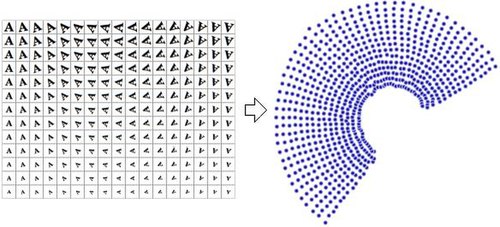
106:(the letter 'A') and recover only the varying information (rotation and scale). The image to the right shows sample images from this dataset (to save space, not all input images are shown), and a plot of the two-dimensional points that results from using a NLDR algorithm (in this case, Manifold Sculpting was used) to reduce the data into just two dimensions.
640:). The graph thus generated can be considered as a discrete approximation of the low-dimensional manifold in the high-dimensional space. Minimization of a cost function based on the graph ensures that points close to each other on the manifold are mapped close to each other in the low-dimensional space, preserving local distances. The eigenfunctions of the
668:(MDS). Classic MDS takes a matrix of pair-wise distances between all points and computes a position for each point. Isomap assumes that the pair-wise distances are only known between neighboring points, and uses the Floyd–Warshall algorithm to compute the pair-wise distances between all other points. This effectively estimates the full matrix of pair-wise
697:
technique to find the low-dimensional embedding of points, such that each point is still described with the same linear combination of its neighbors. LLE tends to handle non-uniform sample densities poorly because there is no fixed unit to prevent the weights from drifting as various regions differ in sample densities. LLE has no internal model.
167:
135:. In particular, if there is an attracting invariant manifold in the phase space, nearby trajectories will converge onto it and stay on it indefinitely, rendering it a candidate for dimensionality reduction of the dynamical system. While such manifolds are not guaranteed to exist in general, the theory of
61:, with the goal of either visualizing the data in the low-dimensional space, or learning the mapping (either from the high-dimensional space to the low-dimensional embedding or vice versa) itself. The techniques described below can be understood as generalizations of linear decomposition methods used for
3218:
RankVisu is designed to preserve rank of neighborhood rather than distance. RankVisu is especially useful on difficult tasks (when the preservation of distance cannot be achieved satisfyingly). Indeed, the rank of neighborhood is less informative than distance (ranks can be deduced from distances but
1210:
of the original weights produced by LLE. The creators of this regularised variant are also the authors of Local
Tangent Space Alignment (LTSA), which is implicit in the MLLE formulation when realising that the global optimisation of the orthogonal projections of each weight vector, in-essence, aligns
2807:
defines a random walk on the data set which means that the kernel captures some local geometry of data set. The Markov chain defines fast and slow directions of propagation through the kernel values. As the walk propagates forward in time, the local geometry information aggregates in the same way as
1267:
which is trained to approximate the identity function. That is, it is trained to map from a vector of values to the same vector. When used for dimensionality reduction purposes, one of the hidden layers in the network is limited to contain only a small number of network units. Thus, the network must
121:, which is a linear dimensionality reduction algorithm, is used to reduce this same dataset into two dimensions, the resulting values are not so well organized. This demonstrates that the high-dimensional vectors (each representing a letter 'A') that sample this manifold vary in a non-linear manner.
105:
is two, because two variables (rotation and scale) were varied in order to produce the data. Information about the shape or look of a letter 'A' is not part of the intrinsic variables because it is the same in every instance. Nonlinear dimensionality reduction will discard the correlated information
1331:
algorithm. The algorithm finds a configuration of data points on a manifold by simulating a multi-particle dynamic system on a closed manifold, where data points are mapped to particles and distances (or dissimilarity) between data points represent a repulsive force. As the manifold gradually grows
635:
Traditional techniques like principal component analysis do not consider the intrinsic geometry of the data. Laplacian eigenmaps builds a graph from neighborhood information of the data set. Each data point serves as a node on the graph and connectivity between nodes is governed by the proximity of
81:
High dimensional data can be hard for machines to work with, requiring significant time and space for analysis. It also presents a challenge for humans, since it's hard to visualize or understand data in more than three dimensions. Reducing the dimensionality of a data set, while keep its essential
1463:
It should be noticed that CCA, as an iterative learning algorithm, actually starts with focus on large distances (like the Sammon algorithm), then gradually change focus to small distances. The small distance information will overwrite the large distance information, if compromises between the two
648:
on the unit circle manifold). Attempts to place
Laplacian eigenmaps on solid theoretical ground have met with some success, as under certain nonrestrictive assumptions, the graph Laplacian matrix has been shown to converge to the Laplace–Beltrami operator as the number of points goes to infinity.
1494:
learns a smooth diffeomorphic mapping which transports the data onto a lower-dimensional linear subspace. The methods solves for a smooth time indexed vector field such that flows along the field which start at the data points will end at a lower-dimensional linear subspace, thereby attempting to
1506:
takes advantage of the assumption that disparate data sets produced by similar generating processes will share a similar underlying manifold representation. By learning projections from each original space to the shared manifold, correspondences are recovered and knowledge from one domain can be
612:
in his 1984 thesis, which he formally introduced in 1989. This idea has been explored further by many authors. How to define the "simplicity" of the manifold is problem-dependent, however, it is commonly measured by the intrinsic dimensionality and/or the smoothness of the manifold. Usually, the
696:
algorithms, and better results with many problems. LLE also begins by finding a set of the nearest neighbors of each point. It then computes a set of weights for each point that best describes the point as a linear combination of its neighbors. Finally, it uses an eigenvector-based optimization
124:
It should be apparent, therefore, that NLDR has several applications in the field of computer-vision. For example, consider a robot that uses a camera to navigate in a closed static environment. The images obtained by that camera can be considered to be samples on a manifold in high-dimensional
96:
The reduced-dimensional representations of data are often referred to as "intrinsic variables". This description implies that these are the values from which the data was produced. For example, consider a dataset that contains images of a letter 'A', which has been scaled and rotated by varying
3176:
to train a multi-layer perceptron (MLP) to fit to a manifold. Unlike typical MLP training, which only updates the weights, NLPCA updates both the weights and the inputs. That is, both the weights and inputs are treated as latent values. After training, the latent inputs are a low-dimensional
549:
must be chosen such that it has a known corresponding kernel. Unfortunately, it is not trivial to find a good kernel for a given problem, so KPCA does not yield good results with some problems when using standard kernels. For example, it is known to perform poorly with these kernels on the
2036:
607:
give the natural geometric framework for nonlinear dimensionality reduction and extend the geometric interpretation of PCA by explicitly constructing an embedded manifold, and by encoding using standard geometric projection onto the manifold. This approach was originally proposed by
627:
Laplacian eigenmaps uses spectral techniques to perform dimensionality reduction. This technique relies on the basic assumption that the data lies in a low-dimensional manifold in a high-dimensional space. This algorithm cannot embed out-of-sample points, but techniques based on
1314:(t-SNE) is widely used. It is one of a family of stochastic neighbor embedding methods. The algorithm computes the probability that pairs of datapoints in the high-dimensional space are related, and then chooses low-dimensional embeddings which produce a similar distribution.
613:
principal manifold is defined as a solution to an optimization problem. The objective function includes a quality of data approximation and some penalty terms for the bending of the manifold. The popular initial approximations are generated by linear PCA and
Kohonen's SOM.
485:
1140:
849:
1196:
is also based on sparse matrix techniques. It tends to yield results of a much higher quality than LLE. Unfortunately, it has a very costly computational complexity, so it is not well-suited for heavily sampled manifolds. It has no internal model.
139:
gives conditions for the existence of unique attracting invariant objects in a broad class of dynamical systems. Active research in NLDR seeks to unfold the observation manifolds associated with dynamical systems to develop modeling techniques.
1247:, Isomap and Locally Linear Embedding share a common intuition relying on the notion that if a manifold is properly unfolded, then variance over the points is maximized. Its initial step, like Isomap and Locally Linear Embedding, is finding the
1205:
Modified LLE (MLLE) is another LLE variant which uses multiple weights in each neighborhood to address the local weight matrix conditioning problem which leads to distortions in LLE maps. Loosely speaking the multiple weights are the local
680:
that is embedded inside of a higher-dimensional vector space. The main intuition behind MVU is to exploit the local linearity of manifolds and create a mapping that preserves local neighbourhoods at every point of the underlying manifold.
365:
672:
between all of the points. Isomap then uses classic MDS to compute the reduced-dimensional positions of all the points. Landmark-Isomap is a variant of this algorithm that uses landmarks to increase speed, at the cost of some accuracy.
1530:); an analogy is drawn between the diffusion operator on a manifold and a Markov transition matrix operating on functions defined on the graph whose nodes were sampled from the manifold. In particular, let a data set be represented by
57:, is any of various related techniques that aim to project high-dimensional data, potentially existing across non-linear manifolds which cannot be adequately captured by linear decomposition methods, onto lower-dimensional
1883:
2970:
1622:
3189:
and curvilinear component analysis except that (1) it simultaneously penalizes false neighborhoods and tears by focusing on small distances in both original and output space, and that (2) it accounts for
554:
manifold. However, one can view certain other methods that perform well in such settings (e.g., Laplacian
Eigenmaps, LLE) as special cases of kernel PCA by constructing a data-dependent kernel matrix.
644:
on the manifold serve as the embedding dimensions, since under mild conditions this operator has a countable spectrum that is a basis for square integrable functions on the manifold (compare to
1835:
2315:
2220:
968:
1456:(CCA) looks for the configuration of points in the output space that preserves original distances as much as possible while focusing on small distances in the output space (conversely to
38:) with a rectangular hole in the middle. Top-right: the original 2D manifold used to generate the 3D dataset. Bottom left and right: 2D recoveries of the manifold respectively using the
4728:
S. Lespinats, M. Verleysen, A. Giron, B. Fertil, DD-HDS: a tool for visualization and exploration of high-dimensional data, IEEE Transactions on Neural
Networks 18 (5) (2007) 1265–1279.
92:
Plot of the two-dimensional points that results from using a NLDR algorithm. In this case, Manifold
Sculpting is used to reduce the data into just two dimensions (rotation and scale).
97:
amounts. Each image has 32×32 pixels. Each image can be represented as a vector of 1024 pixel values. Each row is a sample on a two-dimensional manifold in 1024-dimensional space (a
380:
1032:
741:
527:
2852:
2701:
2079:
2533:
1766:
1704:
1644:
273:
3092:
3042:
2462:
692:(LLE) was presented at approximately the same time as Isomap. It has several advantages over Isomap, including faster optimization when implemented to take advantage of
4743:, In Platt, J.C. and Koller, D. and Singer, Y. and Roweis, S., editor, Advances in Neural Information Processing Systems 20, pp. 513–520, MIT Press, Cambridge, MA, 2008
251:
2351:
2256:
2371:
2161:
1228:
is based on the intuition that when a manifold is correctly unfolded, all of the tangent hyperplanes to the manifold will become aligned. It begins by computing the
280:
2353:. The former means that very little diffusion has taken place while the latter implies that the diffusion process is nearly complete. Different strategies to choose
3761:
3146:
3119:
3000:
2728:
2641:
2614:
2587:
2560:
2133:
2106:
1413:
547:
2808:
local transitions (defined by differential equations) of the dynamical system. The metaphor of diffusion arises from the definition of a family diffusion distance
1850:
as defining some sort of affinity on that graph. The graph is symmetric by construction since the kernel is symmetric. It is easy to see here that from the tuple (
1668:
1439:
2805:
2775:
2748:
2484:
2417:
2394:
2143:. Since the exact structure of the manifold is not available, for the nearest neighbors the geodesic distance is approximated by euclidean distance. The choice
374:
eigenvectors of that matrix. By comparison, KPCA begins by computing the covariance matrix of the data after being transformed into a higher-dimensional space,
1311:
1211:
the local tangent spaces of every data point. The theoretical and empirical implications from the correct application of this algorithm are far-reaching.
113:
PCA (a linear dimensionality reduction algorithm) is used to reduce this same dataset into two dimensions, the resulting values are not so well organized.
1507:
transferred to another. Most manifold alignment techniques consider only two data sets, but the concept extends to arbitrarily many initial data sets.
1335:
Relational perspective map was inspired by a physical model in which positively charged particles move freely on the surface of a ball. Guided by the
3891:
2031:{\displaystyle K_{ij}={\begin{cases}e^{-\|x_{i}-x_{j}\|_{2}^{2}/\sigma ^{2}}&{\text{if }}x_{i}\sim x_{j}\\0&{\text{otherwise}}\end{cases}}}
1332:
in size the multi-particle system cools down gradually and converges to a configuration that reflects the distance information of the data points.
3652:
632:
regularization exist for adding this capability. Such techniques can be applied to other nonlinear dimensionality reduction algorithms as well.
3148:
takes into account all the relation between points x and y while calculating the distance and serves as a better notion of proximity than just
4870:
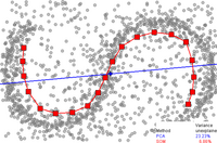
3802:
3568:
3474:
Haller, George; Ponsioen, Sten (2016). "Nonlinear normal modes and spectral submanifolds: Existence, uniqueness and use in model reduction".
3458:
3177:
representation of the observed vectors, and the MLP maps from that low-dimensional representation to the high-dimensional observation space.
2859:
3412:
1342:
between particles, the minimal energy configuration of the particles will reflect the strength of repulsive forces between the particles.
88:
1479:
in its embedding. It is based on
Curvilinear Component Analysis (which extended Sammon's mapping), but uses geodesic distances instead.
224:
1533:
4808:
McInnes, Leland; Healy, John; Melville, James (2018-12-07). "Uniform manifold approximation and projection for dimension reduction".
3906:
3842:
110:
3732:
3242:
Uniform manifold approximation and projection (UMAP) is a nonlinear dimensionality reduction technique. Visually, it is similar to
3227:
2785:
is that only local features of the data are considered in diffusion maps as opposed to taking correlations of the entire data set.
1284:(see above) to learn a non-linear mapping from the high-dimensional to the embedded space. The mappings in NeuroScale are based on
3305:
is an open source C++ library containing implementations of LLE, Manifold
Sculpting, and some other manifold learning algorithms.
629:
183:
4176:
Zhang, Zhenyue; Hongyuan Zha (2005). "Principal
Manifolds and Nonlinear Dimension Reduction via Local Tangent Space Alignment".
3627:
Ham, Jihun; Lee, Daniel D.; Mika, Sebastian; Schölkopf, Bernhard. "A kernel view of the dimensionality reduction of manifolds".
1236:-first principal components in each local neighborhood. It then optimizes to find an embedding that aligns the tangent spaces.
3650:
Gorban, A. N.; Zinovyev, A. (2010). "Principal manifolds and graphs in practice: from molecular biology to dynamical systems".
1624:. The underlying assumption of diffusion map is that the high-dimensional data lies on a low-dimensional manifold of dimension
4926:
4222:
1161:
211:
based on a non-linear mapping from the embedded space to the high-dimensional space. These techniques are related to work on
204:
4921:
1296:
641:
4916:
3323:
1285:
1225:
1220:
661:
557:
KPCA has an internal model, so it can be used to map points onto its embedding that were not available at training time.
4946:
3788:
3312:
2782:
1269:
637:
179:
118:
70:
66:
4767:
3890:
Bengio, Yoshua; Paiement, Jean-Francois; Vincent, Pascal; Delalleau, Olivier; Le Roux, Nicolas; Ouimet, Marie (2004).
3379:
1780:
1336:
4901:
2261:
2166:
1453:
923:
82:
features relatively intact, can make algorithms more efficient and allow analysts to visualize trends and patterns.
3286:
1244:
3359:
3282:
1172:
nonzero eigen vectors provide an orthogonal set of coordinates. Generally the data points are reconstructed from
589:
incidence. Different forms and colors correspond to various geographical locations. Red bold line represents the
498:
to factor away much of the computation, such that the entire process can be performed without actually computing
4519:
3274:
3191:
3161:
1328:
1277:
665:
62:
4891:
3923:
689:
480:{\displaystyle C={\frac {1}{m}}\sum _{i=1}^{m}{\Phi (\mathbf {x} _{i})\Phi (\mathbf {x} _{i})^{\mathsf {T}}}.}
17:
4455:
3709:
1135:{\displaystyle C(Y)=\sum _{i}\left|\mathbf {Y} _{i}-\sum _{j}{\mathbf {W} _{ij}\mathbf {Y} _{j}}\right|^{2}}
844:{\displaystyle E(W)=\sum _{i}\left|\mathbf {X} _{i}-\sum _{j}{\mathbf {W} _{ij}\mathbf {X} _{j}}\right|^{2}}
622:
4384:
Taylor, D.; Klimm, F.; Harrington, H. A.; Kramár, M.; Mischaikow, K.; Porter, M. A.; Mucha, P. J. (2015).
4185:
3585:
3290:
3265:
A method based on proximity matrices is one where the data is presented to the algorithm in the form of a
3203:
1373:
Contagion maps use multiple contagions on a network to map the nodes as a point cloud. In the case of the
574:
4886:
501:
125:
space, and the intrinsic variables of that manifold will represent the robot's position and orientation.
4585:
3364:
2811:
2650:
1374:
1207:
208:
4830:"UMAP: Uniform Manifold Approximation and Projection for Dimension Reduction — umap 0.3 documentation"
4753:
4497:
4343:
3541:
212:
4627:
4456:"Curvilinear Component Analysis: A Self-Organizing Neural Network for Nonlinear Mapping of Data Sets"
4407:
4317:
4044:
3989:
3980:
Roweis, S. T.; Saul, L. K. (2000). "Nonlinear
Dimensionality Reduction by Locally Linear Embedding".
3938:
3878:
3870:
3431:
3408:"A unifying probabilistic perspective for spectral dimensionality reduction: insights and new models"
3349:
2044:
602:
136:
4248:"Probabilistic Non-linear Principal Component Analysis with Gaussian Process Latent Variable Models"
4190:
2489:
1908:
1712:
3385:
3354:
3344:
3250:
3231:
3186:
3002:
defines a distance between any two points of the data set based on path connectivity: the value of
1685:
1457:
196:
171:
160:
102:
4096:
NIPS'06: Proceedings of the 19th International Conference on Neural Information Processing Systems
3528:. Proceedings of the International Joint Conference on Neural Networks IJCNN'11. pp. 1959–66.
1627:
1232:-nearest neighbors of every point. It computes the tangent space at every point by computing the
256:
4809:
4790:
4608:
4397:
4366:
4298:
4158:
4122:
4013:
3962:
3687:
3661:
3609:
3501:
3483:
3421:
3149:
1503:
1193:
1177:
128:
3823:
3055:
3005:
2425:
1273:
360:{\displaystyle C={\frac {1}{m}}\sum _{i=1}^{m}{\mathbf {x} _{i}\mathbf {x} _{i}^{\mathsf {T}}}.}
3753:
3319:
569:
Application of principal curves: Nonlinear quality of life index. Points represent data of the
230:
4866:
4858:
4711:
4660:
4478:
4433:
4290:
4228:
4218:
4150:
4072:
4005:
3954:
3902:
3848:
3838:
3798:
3679:
3564:
3454:
3266:
3254:
3247:
2320:
2225:
1476:
669:
132:
3563:. Lecture Notes in Computer Science and Engineering. Vol. 58. Springer. pp. 68–95.
2356:
2146:
4911:
4782:
4701:
4691:
4652:
4600:
4470:
4423:
4415:
4358:
4282:
4195:
4140:
4132:
4062:
4052:
3997:
3946:
3770:
3671:
3632:
3601:
3493:
3374:
3277:. The variations tend to be differences in how the proximity data is computed; for example,
1358:
1339:
1300:
1010:
dimensional space. A neighborhood preserving map is created based on this idea. Each point X
582:
4386:"Topological data analysis of contagion maps for examining spreading processes on networks"
3124:
3097:
2978:
2706:
2619:
2592:
2565:
2538:
2111:
2084:
1380:
532:
182:
is presented by a blue straight line. Data points are the small grey circles. For PCA, the
4706:
4567:
4541:
3293:(which is not in fact a mapping) are examples of metric multidimensional scaling methods.
3270:
3173:
1653:
718:. The original point is reconstructed by a linear combination, given by the weight matrix
578:
58:
3629:
Proceedings of the 21st International Conference on Machine Learning, Banff, Canada, 2004
1418:
1153:
to optimize the coordinates. This minimization problem can be solved by solving a sparse
4411:
4048:
3993:
3942:
3723:
3435:
1846:
Thus one can think of the individual data points as the nodes of a graph and the kernel
4428:
4385:
4247:
4145:
4110:
2790:
2760:
2733:
2469:
2402:
2379:
1862:. This technique is common to a variety of fields and is known as the graph Laplacian.
1281:
1264:
645:
570:
4067:
4032:
3520:
1475:
CDA trains a self-organizing neural network to fit the manifold and seeks to preserve
1345:
The Relational perspective map was introduced in. The algorithm firstly used the flat
4940:
4768:"Nonlinear Dimensionality Reduction by Topologically Constrained Isometric Embedding"
4162:
4091:
3966:
3819:
3797:. Lecture Notes in Computer Science and Engineering (LNCSE). Vol. 58. Springer.
3792:
3749:
2397:
1515:
1487:
693:
676:
In manifold learning, the input data is assumed to be sampled from a low dimensional
609:
495:
98:
4739:
4696:
4679:
4612:
4302:
3505:
3164:
in local regions, and then uses convex optimization to fit all the pieces together.
4794:
4370:
4111:"Locally Linear Embedding and fMRI feature selection in psychiatric classification"
4017:
3892:"Out-of-Sample Extensions for LLE, Isomap, MDS, Eigenmaps, and Spectral Clustering"
3774:
3705:
3691:
3613:
1859:
1527:
1362:
977:
dimensional space and the goal of the algorithm is to reduce the dimensionality to
586:
4033:"Hessian eigenmaps: Locally linear embedding techniques for high-dimensional data"
4001:
3950:
3407:
30:
4656:
4561:
4362:
3369:
1523:
1260:
594:
593:, approximating the dataset. This principal curve was produced by the method of
175:
4829:
4604:
4270:
4136:
3605:
3308:
565:
4786:
4286:
4199:
3675:
3497:
551:
35:
4232:
3219:
distances cannot be deduced from ranks) and its preservation is thus easier.
1467:
The stress function of CCA is related to a sum of right Bregman divergences.
4057:
3852:
3636:
3597:
3194:
phenomenon by adapting the weighting function to the distance distribution.
1519:
881:. The cost function is minimized under two constraints: (a) Each data point
4715:
4664:
4482:
4437:
4294:
4154:
4076:
4009:
3958:
3683:
727:, of its neighbors. The reconstruction error is given by the cost function
573:
171 countries in 4-dimensional space formed by the values of 4 indicators:
4213:
DeMers, D.; Cottrell, G.W. (1993). "Non-linear dimensionality reduction".
3824:"Laplacian Eigenmaps and Spectral Techniques for Embedding and Clustering"
1495:
preserve pairwise differences under both the forward and inverse mapping.
1006:
dimensional space will be used to reconstruct the same point in the lower
4906:
4549:. The 25th International Conference on Machine Learning. pp. 1120–7.
2140:
2136:
677:
4896:
109:
4419:
3588:(1998). "Nonlinear Component Analysis as a Kernel Eigenvalue Problem".
3556:
1180:. For such an implementation the algorithm has only one free parameter
4474:
2965:{\displaystyle D_{t}^{2}(x,y)=\|p_{t}(x,\cdot )-p_{t}(y,\cdot )\|^{2}}
34:
Top-left: a 3D dataset of 1000 points in a spiraling band (a.k.a. the
4740:
Iterative Non-linear Dimensionality Reduction with Manifold Sculpting
4271:"Multilayer Joint Gait-Pose Manifolds for Human Gait Motion Modeling"
3924:"A Global Geometric Framework for Nonlinear Dimensionality Reduction"
3331:
3278:
1442:
1377:
the speed of the spread can be adjusted with the threshold parameter
1354:
657:
3185:
Data-driven high-dimensional scaling (DD-HDS) is closely related to
223:
Perhaps the most widely used algorithm for dimensional reduction is
4814:
4344:"Visualizing high-dimensional data with relational perspective map"
4127:
3557:"3. Learning Nonlinear Principal Manifolds by Self-Organising Maps"
3488:
3327:
1272:
and stacked denoising autoencoders. Related to autoencoders is the
166:
43:
4678:
Scholz, M.; Kaplan, F.; Guy, C. L.; Kopka, J.; Selbig, J. (2005).
4402:
3877:
Matlab code for Laplacian Eigenmaps can be found in algorithms at
3794:
Principal Manifolds for Data Visualisation and Dimension Reduction
3666:
3561:
Principal Manifolds for Data Visualization and Dimension Reduction
3426:
3302:
2589:
in one time step. Similarly the probability of transitioning from
1349:
as the image manifold, then it has been extended (in the software
1346:
165:
108:
87:
29:
4766:
Rosman, G.; Bronstein, M.M.; Bronstein, A.M.; Kimmel, R. (2010).
3121:
is much more robust to noise in the data than geodesic distance.
207:(GTM) use a point representation in the embedded space to form a
46:
algorithms as implemented by the Modular Data Processing toolkit.
4115:
IEEE Journal of Translational Engineering in Health and Medicine
4092:"MLLE: Modified Locally Linear Embedding Using Multiple Weights"
3731:(PhD). Stanford Linear Accelerator Center, Stanford University.
3559:. In Gorban, A.N.; Kégl, B.; Wunsch, D.C.; Zinovyev, A. (eds.).
3243:
1617:{\displaystyle \mathbf {X} =\in \Omega \subset \mathbf {R^{D}} }
4643:
Venna, J.; Kaski, S. (2006). "Local multidimensional scaling".
3542:"Principal Component Analysis and Self-Organizing Maps: applet"
3246:, but it assumes that the data is uniformly distributed on a
3206:
to find an embedding. Like other algorithms, it computes the
2139:
distance should be used to actually measure distances on the
1145:
In this cost function, unlike the previous one, the weights W
917:
and (b) The sum of every row of the weight matrix equals 1.
3875:(PhD). Department of Mathematics, The University of Chicago.
1691:
215:, which also are based around the same probabilistic model.
2024:
1149:
are kept fixed and the minimization is done on the points Y
2777:
constitutes some notion of local geometry of the data set
1678:
which represents some notion of affinity of the points in
1350:
890:
is reconstructed only from its neighbors, thus enforcing
4931:
4505:
European Symposium on Artificial Neural Networks (Esann)
4498:"Curvilinear component analysis and Bregman divergences"
494:
eigenvectors of that matrix, just like PCA. It uses the
4756:, Neurocomputing, vol. 72 (13–15), pp. 2964–2978, 2009.
3257:
is locally constant or approximately locally constant.
2163:
modulates our notion of proximity in the sense that if
227:. PCA begins by computing the covariance matrix of the
4752:
Lespinats S., Fertil B., Villemain P. and Herault J.,
3922:
Tenenbaum, J B.; de Silva, V.; Langford, J.C. (2000).
3791:; Kégl, B.; Wunsch, D. C.; Zinovyev, A., eds. (2007).
170:
Approximation of a principal curve by one-dimensional
163:
is one of the first and most popular NLDR techniques.
3127:
3100:
3058:
3008:
2981:
2862:
2814:
2793:
2763:
2736:
2709:
2653:
2622:
2595:
2568:
2541:
2492:
2472:
2428:
2405:
2382:
2359:
2323:
2264:
2228:
2169:
2149:
2114:
2087:
2047:
1886:
1783:
1715:
1688:
1656:
1630:
1536:
1421:
1383:
1035:
926:
744:
535:
504:
490:
It then projects the transformed data onto the first
383:
283:
259:
233:
131:
are of general interest for model order reduction in
3273:. These methods all fall under the broader class of
700:
LLE computes the barycentric coordinates of a point
3311:implements the method for the programming language
1460:which focus on small distances in original space).
1276:algorithm, which uses stress functions inspired by
27:
Projection of data onto lower-dimensional manifolds
3538:The illustration is prepared using free software:
3140:
3113:
3086:
3036:
2994:
2964:
2846:
2799:
2781:. The major difference between diffusion maps and
2769:
2742:
2722:
2695:
2635:
2608:
2581:
2554:
2527:
2478:
2456:
2411:
2388:
2376:In order to faithfully represent a Markov matrix,
2365:
2345:
2309:
2250:
2214:
2155:
2127:
2100:
2073:
2030:
1829:
1760:
1698:
1662:
1638:
1616:
1433:
1407:
1134:
1026:dimensional space by minimizing the cost function
962:
843:
541:
521:
479:
359:
267:
245:
4584:Coifman, Ronald R.; Lafon, Stephane (July 2006).
4527:Advances in Neural Information Processing Systems
4496:Sun, Jigang; Crowe, Malcolm; Fyfe, Colin (2010).
4215:Advances in neural information processing systems
3899:Advances in Neural Information Processing Systems
3831:Advances in Neural Information Processing Systems
1670:represent the distribution of the data points on
1353:to use other types of closed manifolds, like the
4754:Rankvisu: Mapping from the neighbourhood network
1830:{\displaystyle k(x,y)\geq 0\qquad \forall x,y,k}
4518:Walder, Christian; Schölkopf, Bernhard (2009).
4318:"Visualizing High-Dimensional Data Using t-SNE"
3762:Journal of the American Statistical Association
1168:being the number of data points), whose bottom
186:in this example is 23.23%, for SOM it is 6.86%.
4737:Gashler, M. and Ventura, D. and Martinez, T.,
3094:involves a sum over of all paths of length t,
2310:{\displaystyle \|x_{i}-x_{j}\|_{2}\ll \sigma }
2215:{\displaystyle \|x_{i}-x_{j}\|_{2}\gg \sigma }
1877:) can be constructed using a Gaussian kernel.
1188:Hessian locally-linear embedding (Hessian LLE)
963:{\displaystyle \sum _{j}{\mathbf {W} _{ij}}=1}
863:refer to the amount of contribution the point
4579:
4577:
4540:Wang, Chang; Mahadevan, Sridhar (July 2008).
4316:van der Maaten, L.J.P.; Hinton, G.E. (2008).
3238:Uniform manifold approximation and projection
3228:Topologically constrained isometric embedding
3223:Topologically constrained isometric embedding
39:
18:Uniform Manifold Approximation and Projection
8:
4932:Nonlinear PCA by autoencoder neural networks
4543:Manifold Alignment using Procrustes Analysis
4529:. Vol. 22. MIT Press. pp. 1713–20.
3044:will be smaller the more paths that connect
2953:
2896:
2829:
2815:
2292:
2265:
2197:
2170:
1946:
1919:
973:The original data points are collected in a
4593:Applied and Computational Harmonic Analysis
3708:- Multidimensional Data Visualization Tool
3522:Temporal Nonlinear Dimensionality Reduction
1312:t-distributed stochastic neighbor embedding
1307:t-distributed stochastic neighbor embedding
1018:dimensional space is mapped onto a point Y
4813:
4705:
4695:
4680:"Non-linear PCA: a missing data approach"
4629:Diffusion Maps: Applications and Analysis
4449:
4447:
4427:
4401:
4189:
4144:
4126:
4066:
4056:
3864:
3862:
3665:
3487:
3425:
3132:
3126:
3105:
3099:
3063:
3057:
3013:
3007:
2986:
2980:
2956:
2931:
2903:
2872:
2867:
2861:
2832:
2822:
2813:
2792:
2762:
2735:
2714:
2708:
2684:
2671:
2658:
2652:
2627:
2621:
2600:
2594:
2573:
2567:
2546:
2540:
2535:is the probability of transitioning from
2516:
2503:
2491:
2471:
2439:
2427:
2404:
2381:
2358:
2328:
2322:
2295:
2285:
2272:
2263:
2233:
2227:
2200:
2190:
2177:
2168:
2148:
2119:
2113:
2092:
2086:
2065:
2052:
2046:
2016:
2001:
1988:
1979:
1969:
1960:
1954:
1949:
1939:
1926:
1915:
1903:
1891:
1885:
1782:
1714:
1690:
1689:
1687:
1655:
1631:
1629:
1607:
1602:
1584:
1565:
1552:
1537:
1535:
1420:
1382:
1184:which can be chosen by cross validation.
1126:
1114:
1109:
1099:
1094:
1092:
1086:
1073:
1068:
1055:
1034:
944:
939:
937:
931:
925:
835:
823:
818:
808:
803:
801:
795:
782:
777:
764:
743:
534:
511:
503:
466:
465:
455:
450:
434:
429:
421:
415:
404:
390:
382:
370:It then projects the data onto the first
346:
345:
340:
335:
328:
323:
321:
315:
304:
290:
282:
260:
258:
232:
4775:International Journal of Computer Vision
4690:(20). Oxford University Press: 3887–95.
4520:"Diffeomorphic Dimensionality Reduction"
3449:Lee, John A.; Verleysen, Michel (2007).
3160:Local Multidimensional Scaling performs
2396:must be normalized by the corresponding
1518:leverages the relationship between heat
1201:Modified Locally-Linear Embedding (MLLE)
564:
3653:International Journal of Neural Systems
3398:
1441:the contagion map is equivalent to the
1297:Gaussian process latent variable models
1292:Gaussian process latent variable models
178:with red squares, 20 nodes). The first
4902:Gaussian Process Latent Variable Model
4563:Diffusion Maps and Geometric Harmonics
4507:. d-side publications. pp. 81–86.
1483:Diffeomorphic dimensionality reduction
467:
347:
3052:and vice versa. Because the quantity
7:
4463:IEEE Transactions on Neural Networks
4454:Demartines, P.; Hérault, J. (1997).
4325:Journal of Machine Learning Research
4252:Journal of Machine Learning Research
4178:SIAM Journal on Scientific Computing
3738:from the original on August 2, 2019.
3413:Journal of Machine Learning Research
3181:Data-driven high-dimensional scaling
3261:Methods based on proximity matrices
872:has while reconstructing the point
636:neighboring points (using e.g. the
522:{\displaystyle \Phi (\mathbf {x} )}
219:Kernel principal component analysis
3519:Gashler, M.; Martinez, T. (2011).
3451:Nonlinear Dimensionality Reduction
2847:{\displaystyle \{D_{t}\}_{t\in N}}
2696:{\displaystyle P^{t}(x_{i},x_{j})}
1809:
1596:
1176:nearest neighbors, as measured by
536:
505:
443:
422:
145:nonlinear dimensionality reduction
51:Nonlinear dimensionality reduction
25:
3872:Problems of Learning on Manifolds
1858:) one can construct a reversible
4632:(Masters). University of Oxford.
4275:IEEE Transactions on Cybernetics
1632:
1608:
1604:
1538:
1327:Relational perspective map is a
1110:
1095:
1069:
940:
819:
804:
778:
630:Reproducing kernel Hilbert space
512:
451:
430:
336:
324:
261:
203:) and its probabilistic variant
184:Fraction of variance unexplained
4865:. MIT Press. pp. 682–699.
4217:. Vol. 5. pp. 580–7.
4031:Donoho, D.; Grimes, C. (2003).
3869:Belkin, Mikhail (August 2003).
3275:metric multidimensional scaling
2486:now represents a Markov chain.
2074:{\displaystyle x_{i}\sim x_{j}}
1808:
908:is not a neighbor of the point
4927:Short review of Diffusion Maps
4892:Generative Topographic Mapping
4863:Probabilistic Machine Learning
4707:11858/00-001M-0000-0014-2B1F-2
3775:10.1080/01621459.1989.10478797
3156:Local multidimensional scaling
3081:
3069:
3031:
3019:
2949:
2937:
2921:
2909:
2890:
2878:
2690:
2664:
2528:{\displaystyle P(x_{i},x_{j})}
2522:
2496:
1799:
1787:
1761:{\displaystyle k(x,y)=k(y,x),}
1752:
1740:
1731:
1719:
1590:
1545:
1454:Curvilinear component analysis
1449:Curvilinear component analysis
1402:
1390:
1286:radial basis function networks
1045:
1039:
754:
748:
561:Principal curves and manifolds
516:
508:
462:
446:
440:
425:
205:generative topographic mapping
1:
4697:10.1093/bioinformatics/bti634
4002:10.1126/science.290.5500.2323
3951:10.1126/science.290.5500.2319
3725:Principal Curves and Surfaces
1706:has the following properties
1699:{\displaystyle {\mathit {k}}}
1471:Curvilinear distance analysis
1270:restricted Boltzmann machines
1221:Local tangent space alignment
1215:Local tangent space alignment
147:techniques are listed below.
4657:10.1016/j.neunet.2006.05.014
4560:Lafon, Stephane (May 2004).
4363:10.1057/palgrave.ivs.9500051
4090:Zhang, Z.; Wang, J. (2006).
3752:; Stuetzle, W. (June 1989).
3722:Hastie, T. (November 1984).
2783:principal component analysis
1639:{\displaystyle \mathbf {d} }
1490:Dimensionality Reduction or
638:k-nearest neighbor algorithm
268:{\displaystyle \mathbf {X} }
119:principal component analysis
71:principal component analysis
67:singular value decomposition
3901:. Vol. 16. MIT Press.
3380:Growing self-organizing map
3172:Nonlinear PCA (NLPCA) uses
3152:or even geodesic distance.
1650:represent the data set and
143:Some of the more prominent
137:spectral submanifolds (SSM)
4963:
4912:Relational Perspective Map
4605:10.1016/j.acha.2006.04.006
4269:Ding, M.; Fan, G. (2015).
4137:10.1109/JTEHM.2019.2936348
3606:10.1162/089976698300017467
3584:Schölkopf, B.; Smola, A.;
3544:. University of Leicester.
3287:maximum variance unfolding
3087:{\displaystyle D_{t}(x,y)}
3037:{\displaystyle D_{t}(x,y)}
2457:{\displaystyle P=D^{-1}K.}
1323:Relational perspective map
1245:Maximum Variance Unfolding
1240:Maximum variance unfolding
1218:
620:
4857:Murphy, Kevin P. (2022).
4834:umap-learn.readthedocs.io
4787:10.1007/s11263-010-0322-1
4351:Information Visualization
4287:10.1109/TCYB.2014.2373393
4200:10.1137/s1064827502419154
3676:10.1142/S0129065710002383
3498:10.1007/s11071-016-2974-z
3406:Lawrence, Neil D (2012).
3360:Whitney embedding theorem
3283:locally linear embeddings
2108:is a nearest neighbor of
1843:is positivity preserving
642:Laplace–Beltrami operator
246:{\displaystyle m\times n}
4907:Locally Linear Embedding
4037:Proc Natl Acad Sci U S A
3202:Manifold Sculpting uses
3192:concentration of measure
3162:multidimensional scaling
2346:{\displaystyle K_{ij}=1}
2251:{\displaystyle K_{ij}=0}
1329:multidimensional scaling
1278:multidimensional scaling
690:Locally-linear Embedding
685:Locally-linear embedding
666:Multidimensional Scaling
662:Floyd–Warshall algorithm
660:is a combination of the
575:gross product per capita
103:intrinsic dimensionality
63:dimensionality reduction
4058:10.1073/pnas.1031596100
3637:10.1145/1015330.1015417
2647:time steps is given by
2366:{\displaystyle \sigma }
2156:{\displaystyle \sigma }
2041:In the above equation,
1865:For example, the graph
709:based on its neighbors
623:Manifold regularization
155:
3837:. MIT Press: 586–691.
3204:graduated optimization
3142:
3115:
3088:
3038:
2996:
2966:
2848:
2801:
2771:
2744:
2724:
2697:
2637:
2610:
2583:
2556:
2529:
2480:
2458:
2413:
2390:
2367:
2347:
2311:
2252:
2216:
2157:
2129:
2102:
2075:
2032:
1831:
1762:
1700:
1664:
1640:
1618:
1435:
1409:
1365:, as image manifolds.
1136:
998:that reconstructs the
964:
845:
598:
543:
523:
481:
420:
361:
320:
269:
247:
187:
114:
93:
47:
4897:Mike Tipping's Thesis
4390:Nature Communications
4342:Li, James X. (2004).
4246:Lawrence, N. (2005).
4109:Sidhu, Gagan (2019).
3540:Mirkes, E.M. (2011).
3365:Discriminant analysis
3143:
3141:{\displaystyle D_{t}}
3116:
3114:{\displaystyle D_{t}}
3089:
3039:
2997:
2995:{\displaystyle D_{t}}
2967:
2849:
2802:
2772:
2750:multiplied by itself
2745:
2725:
2723:{\displaystyle P^{t}}
2698:
2638:
2636:{\displaystyle x_{j}}
2611:
2609:{\displaystyle x_{i}}
2584:
2582:{\displaystyle x_{j}}
2557:
2555:{\displaystyle x_{i}}
2530:
2481:
2459:
2414:
2391:
2368:
2348:
2312:
2253:
2217:
2158:
2130:
2128:{\displaystyle x_{j}}
2103:
2101:{\displaystyle x_{i}}
2076:
2033:
1832:
1763:
1701:
1665:
1641:
1619:
1436:
1410:
1408:{\displaystyle t\in }
1375:Global cascades model
1208:orthogonal projection
1137:
1002:th data point in the
965:
846:
568:
544:
542:{\displaystyle \Phi }
524:
482:
400:
362:
300:
270:
248:
209:latent variable model
169:
112:
91:
33:
3350:Spectral submanifold
3318:The method has also
3125:
3098:
3056:
3006:
2979:
2860:
2812:
2791:
2761:
2734:
2707:
2651:
2620:
2593:
2566:
2539:
2490:
2470:
2426:
2403:
2380:
2357:
2321:
2262:
2226:
2167:
2147:
2112:
2085:
2045:
1884:
1781:
1713:
1686:
1674:. Further, define a
1663:{\displaystyle \mu }
1654:
1628:
1534:
1419:
1381:
1033:
924:
899:to be zero if point
742:
533:
502:
381:
281:
257:
231:
77:Applications of NLDR
4947:Dimension reduction
4859:"Manifold Learning"
4412:2015NatCo...6.7723T
4049:2003PNAS..100.5591D
3994:2000Sci...290.2323R
3943:2000Sci...290.2319T
3555:Yin, Hujun (2007).
3436:2010arXiv1010.4830L
3386:Self-organizing map
3345:Manifold hypothesis
3251:Riemannian manifold
3232:stress majorization
2877:
1959:
1434:{\displaystyle t=0}
1162:eigen value problem
989:. The same weights
617:Laplacian eigenmaps
352:
197:self-organizing map
191:Self-organizing map
180:principal component
129:Invariant manifolds
4420:10.1038/ncomms8723
3754:"Principal Curves"
3590:Neural Computation
3476:Nonlinear Dynamics
3198:Manifold sculpting
3150:Euclidean distance
3138:
3111:
3084:
3034:
2992:
2962:
2863:
2844:
2797:
2767:
2757:The Markov matrix
2740:
2720:
2693:
2633:
2606:
2579:
2552:
2525:
2476:
2454:
2409:
2386:
2363:
2343:
2307:
2248:
2212:
2153:
2125:
2098:
2071:
2028:
2023:
1945:
1827:
1758:
1696:
1660:
1636:
1614:
1504:Manifold alignment
1499:Manifold alignment
1477:geodesic distances
1431:
1405:
1263:is a feed-forward
1178:Euclidean distance
1132:
1091:
1060:
960:
936:
841:
800:
769:
670:geodesic distances
599:
539:
519:
477:
357:
334:
265:
243:
199:(SOM, also called
188:
151:Important concepts
117:By comparison, if
115:
94:
48:
4922:RankVisu homepage
4872:978-0-262-04682-4
4475:10.1109/72.554199
3937:(5500): 2319–23.
3818:Belkin, Mikhail;
3804:978-3-540-73749-0
3570:978-3-540-73749-0
3460:978-0-387-39350-6
3267:similarity matrix
3255:Riemannian metric
3248:locally connected
2800:{\displaystyle K}
2770:{\displaystyle P}
2743:{\displaystyle P}
2479:{\displaystyle P}
2412:{\displaystyle D}
2389:{\displaystyle K}
2373:can be found in.
2019:
1982:
1464:have to be made.
1082:
1051:
927:
791:
760:
398:
298:
133:dynamical systems
55:manifold learning
16:(Redirected from
4954:
4876:
4844:
4843:
4841:
4840:
4826:
4820:
4819:
4817:
4805:
4799:
4798:
4772:
4763:
4757:
4750:
4744:
4735:
4729:
4726:
4720:
4719:
4709:
4699:
4675:
4669:
4668:
4651:(6–7): 889–899.
4640:
4634:
4633:
4626:Bah, B. (2008).
4623:
4617:
4616:
4590:
4586:"Diffusion Maps"
4581:
4572:
4571:
4557:
4551:
4550:
4548:
4537:
4531:
4530:
4524:
4515:
4509:
4508:
4502:
4493:
4487:
4486:
4460:
4451:
4442:
4441:
4431:
4405:
4381:
4375:
4374:
4348:
4339:
4333:
4332:
4322:
4313:
4307:
4306:
4266:
4260:
4259:
4243:
4237:
4236:
4210:
4204:
4203:
4193:
4173:
4167:
4166:
4148:
4130:
4106:
4100:
4099:
4087:
4081:
4080:
4070:
4060:
4028:
4022:
4021:
3988:(5500): 2323–6.
3977:
3971:
3970:
3928:
3919:
3913:
3912:
3896:
3887:
3881:
3876:
3866:
3857:
3856:
3828:
3815:
3809:
3808:
3785:
3779:
3778:
3758:
3746:
3740:
3739:
3737:
3730:
3719:
3713:
3702:
3696:
3695:
3669:
3647:
3641:
3640:
3624:
3618:
3617:
3581:
3575:
3574:
3552:
3546:
3545:
3536:
3530:
3529:
3527:
3516:
3510:
3509:
3491:
3482:(3): 1493–1534.
3471:
3465:
3464:
3446:
3440:
3439:
3429:
3420:(May): 1609–38.
3403:
3375:Feature learning
3320:been implemented
3187:Sammon's mapping
3147:
3145:
3144:
3139:
3137:
3136:
3120:
3118:
3117:
3112:
3110:
3109:
3093:
3091:
3090:
3085:
3068:
3067:
3043:
3041:
3040:
3035:
3018:
3017:
3001:
2999:
2998:
2993:
2991:
2990:
2971:
2969:
2968:
2963:
2961:
2960:
2936:
2935:
2908:
2907:
2876:
2871:
2853:
2851:
2850:
2845:
2843:
2842:
2827:
2826:
2806:
2804:
2803:
2798:
2776:
2774:
2773:
2768:
2749:
2747:
2746:
2741:
2729:
2727:
2726:
2721:
2719:
2718:
2702:
2700:
2699:
2694:
2689:
2688:
2676:
2675:
2663:
2662:
2642:
2640:
2639:
2634:
2632:
2631:
2615:
2613:
2612:
2607:
2605:
2604:
2588:
2586:
2585:
2580:
2578:
2577:
2561:
2559:
2558:
2553:
2551:
2550:
2534:
2532:
2531:
2526:
2521:
2520:
2508:
2507:
2485:
2483:
2482:
2477:
2463:
2461:
2460:
2455:
2447:
2446:
2418:
2416:
2415:
2410:
2395:
2393:
2392:
2387:
2372:
2370:
2369:
2364:
2352:
2350:
2349:
2344:
2336:
2335:
2316:
2314:
2313:
2308:
2300:
2299:
2290:
2289:
2277:
2276:
2257:
2255:
2254:
2249:
2241:
2240:
2221:
2219:
2218:
2213:
2205:
2204:
2195:
2194:
2182:
2181:
2162:
2160:
2159:
2154:
2134:
2132:
2131:
2126:
2124:
2123:
2107:
2105:
2104:
2099:
2097:
2096:
2080:
2078:
2077:
2072:
2070:
2069:
2057:
2056:
2037:
2035:
2034:
2029:
2027:
2026:
2020:
2017:
2006:
2005:
1993:
1992:
1983:
1980:
1976:
1975:
1974:
1973:
1964:
1958:
1953:
1944:
1943:
1931:
1930:
1899:
1898:
1836:
1834:
1833:
1828:
1767:
1765:
1764:
1759:
1705:
1703:
1702:
1697:
1695:
1694:
1669:
1667:
1666:
1661:
1645:
1643:
1642:
1637:
1635:
1623:
1621:
1620:
1615:
1613:
1612:
1611:
1589:
1588:
1570:
1569:
1557:
1556:
1541:
1458:Sammon's mapping
1440:
1438:
1437:
1432:
1414:
1412:
1411:
1406:
1359:projective space
1318:Other algorithms
1301:Gaussian process
1141:
1139:
1138:
1133:
1131:
1130:
1125:
1121:
1120:
1119:
1118:
1113:
1107:
1106:
1098:
1090:
1078:
1077:
1072:
1059:
969:
967:
966:
961:
953:
952:
951:
943:
935:
850:
848:
847:
842:
840:
839:
834:
830:
829:
828:
827:
822:
816:
815:
807:
799:
787:
786:
781:
768:
603:Principal curves
583:infant mortality
548:
546:
545:
540:
528:
526:
525:
520:
515:
486:
484:
483:
478:
473:
472:
471:
470:
460:
459:
454:
439:
438:
433:
419:
414:
399:
391:
366:
364:
363:
358:
353:
351:
350:
344:
339:
333:
332:
327:
319:
314:
299:
291:
274:
272:
271:
266:
264:
252:
250:
249:
244:
213:density networks
161:Sammon's mapping
156:Sammon's mapping
59:latent manifolds
53:, also known as
21:
4962:
4961:
4957:
4956:
4955:
4953:
4952:
4951:
4937:
4936:
4917:DD-HDS homepage
4883:
4873:
4856:
4853:
4851:Further reading
4848:
4847:
4838:
4836:
4828:
4827:
4823:
4807:
4806:
4802:
4770:
4765:
4764:
4760:
4751:
4747:
4736:
4732:
4727:
4723:
4677:
4676:
4672:
4645:Neural Networks
4642:
4641:
4637:
4625:
4624:
4620:
4588:
4583:
4582:
4575:
4568:Yale University
4559:
4558:
4554:
4546:
4539:
4538:
4534:
4522:
4517:
4516:
4512:
4500:
4495:
4494:
4490:
4458:
4453:
4452:
4445:
4383:
4382:
4378:
4346:
4341:
4340:
4336:
4320:
4315:
4314:
4310:
4281:(11): 2413–24.
4268:
4267:
4263:
4245:
4244:
4240:
4225:
4212:
4211:
4207:
4191:10.1.1.211.9957
4175:
4174:
4170:
4108:
4107:
4103:
4089:
4088:
4084:
4030:
4029:
4025:
3979:
3978:
3974:
3926:
3921:
3920:
3916:
3909:
3894:
3889:
3888:
3884:
3868:
3867:
3860:
3845:
3826:
3817:
3816:
3812:
3805:
3787:
3786:
3782:
3756:
3748:
3747:
3743:
3735:
3728:
3721:
3720:
3716:
3703:
3699:
3649:
3648:
3644:
3626:
3625:
3621:
3583:
3582:
3578:
3571:
3554:
3553:
3549:
3539:
3537:
3533:
3525:
3518:
3517:
3513:
3473:
3472:
3468:
3461:
3448:
3447:
3443:
3405:
3404:
3400:
3395:
3355:Taken's theorem
3341:
3299:
3271:distance matrix
3263:
3240:
3225:
3216:
3200:
3183:
3174:backpropagation
3170:
3158:
3128:
3123:
3122:
3101:
3096:
3095:
3059:
3054:
3053:
3009:
3004:
3003:
2982:
2977:
2976:
2952:
2927:
2899:
2858:
2857:
2828:
2818:
2810:
2809:
2789:
2788:
2759:
2758:
2732:
2731:
2710:
2705:
2704:
2680:
2667:
2654:
2649:
2648:
2623:
2618:
2617:
2596:
2591:
2590:
2569:
2564:
2563:
2542:
2537:
2536:
2512:
2499:
2488:
2487:
2468:
2467:
2435:
2424:
2423:
2401:
2400:
2378:
2377:
2355:
2354:
2324:
2319:
2318:
2291:
2281:
2268:
2260:
2259:
2229:
2224:
2223:
2196:
2186:
2173:
2165:
2164:
2145:
2144:
2115:
2110:
2109:
2088:
2083:
2082:
2061:
2048:
2043:
2042:
2022:
2021:
2014:
2008:
2007:
1997:
1984:
1977:
1965:
1935:
1922:
1911:
1904:
1887:
1882:
1881:
1779:
1778:
1711:
1710:
1684:
1683:
1652:
1651:
1626:
1625:
1603:
1580:
1561:
1548:
1532:
1531:
1513:
1501:
1485:
1473:
1451:
1417:
1416:
1379:
1378:
1371:
1325:
1320:
1309:
1294:
1282:Sammon mappings
1257:
1242:
1223:
1217:
1203:
1190:
1152:
1148:
1108:
1093:
1067:
1066:
1062:
1061:
1031:
1030:
1021:
1013:
997:
938:
922:
921:
916:
907:
898:
889:
880:
871:
862:
817:
802:
776:
775:
771:
770:
740:
739:
726:
717:
708:
687:
655:
625:
619:
591:principal curve
579:life expectancy
563:
531:
530:
500:
499:
461:
449:
428:
379:
378:
322:
279:
278:
255:
254:
229:
228:
221:
193:
158:
153:
85:
79:
28:
23:
22:
15:
12:
11:
5:
4960:
4958:
4950:
4949:
4939:
4938:
4935:
4934:
4929:
4924:
4919:
4914:
4909:
4904:
4899:
4894:
4889:
4882:
4881:External links
4879:
4878:
4877:
4871:
4852:
4849:
4846:
4845:
4821:
4800:
4758:
4745:
4730:
4721:
4684:Bioinformatics
4670:
4635:
4618:
4573:
4552:
4532:
4510:
4488:
4469:(1): 148–154.
4443:
4376:
4334:
4308:
4261:
4238:
4223:
4205:
4184:(1): 313–338.
4168:
4101:
4082:
4043:(10): 5591–6.
4023:
3972:
3914:
3907:
3882:
3879:Ohio-state.edu
3858:
3843:
3820:Niyogi, Partha
3810:
3803:
3780:
3769:(406): 502–6.
3741:
3714:
3710:Institut Curie
3697:
3660:(3): 219–232.
3642:
3619:
3576:
3569:
3547:
3531:
3511:
3466:
3459:
3441:
3397:
3396:
3394:
3391:
3390:
3389:
3383:
3377:
3372:
3367:
3362:
3357:
3352:
3347:
3340:
3337:
3336:
3335:
3316:
3306:
3298:
3295:
3291:Sammon mapping
3262:
3259:
3239:
3236:
3234:that follows.
3224:
3221:
3215:
3212:
3199:
3196:
3182:
3179:
3169:
3166:
3157:
3154:
3135:
3131:
3108:
3104:
3083:
3080:
3077:
3074:
3071:
3066:
3062:
3033:
3030:
3027:
3024:
3021:
3016:
3012:
2989:
2985:
2973:
2972:
2959:
2955:
2951:
2948:
2945:
2942:
2939:
2934:
2930:
2926:
2923:
2920:
2917:
2914:
2911:
2906:
2902:
2898:
2895:
2892:
2889:
2886:
2883:
2880:
2875:
2870:
2866:
2841:
2838:
2835:
2831:
2825:
2821:
2817:
2796:
2766:
2739:
2730:is the matrix
2717:
2713:
2692:
2687:
2683:
2679:
2674:
2670:
2666:
2661:
2657:
2630:
2626:
2603:
2599:
2576:
2572:
2549:
2545:
2524:
2519:
2515:
2511:
2506:
2502:
2498:
2495:
2475:
2465:
2464:
2453:
2450:
2445:
2442:
2438:
2434:
2431:
2408:
2385:
2362:
2342:
2339:
2334:
2331:
2327:
2306:
2303:
2298:
2294:
2288:
2284:
2280:
2275:
2271:
2267:
2247:
2244:
2239:
2236:
2232:
2211:
2208:
2203:
2199:
2193:
2189:
2185:
2180:
2176:
2172:
2152:
2122:
2118:
2095:
2091:
2068:
2064:
2060:
2055:
2051:
2039:
2038:
2025:
2015:
2013:
2010:
2009:
2004:
2000:
1996:
1991:
1987:
1978:
1972:
1968:
1963:
1957:
1952:
1948:
1942:
1938:
1934:
1929:
1925:
1921:
1918:
1914:
1910:
1909:
1907:
1902:
1897:
1894:
1890:
1838:
1837:
1826:
1823:
1820:
1817:
1814:
1811:
1807:
1804:
1801:
1798:
1795:
1792:
1789:
1786:
1769:
1768:
1757:
1754:
1751:
1748:
1745:
1742:
1739:
1736:
1733:
1730:
1727:
1724:
1721:
1718:
1693:
1659:
1634:
1610:
1606:
1601:
1598:
1595:
1592:
1587:
1583:
1579:
1576:
1573:
1568:
1564:
1560:
1555:
1551:
1547:
1544:
1540:
1516:Diffusion maps
1512:
1511:Diffusion maps
1509:
1500:
1497:
1484:
1481:
1472:
1469:
1450:
1447:
1430:
1427:
1424:
1404:
1401:
1398:
1395:
1392:
1389:
1386:
1370:
1369:Contagion maps
1367:
1324:
1321:
1319:
1316:
1308:
1305:
1293:
1290:
1265:neural network
1256:
1253:
1241:
1238:
1219:Main article:
1216:
1213:
1202:
1199:
1189:
1186:
1150:
1146:
1143:
1142:
1129:
1124:
1117:
1112:
1105:
1102:
1097:
1089:
1085:
1081:
1076:
1071:
1065:
1058:
1054:
1050:
1047:
1044:
1041:
1038:
1019:
1011:
993:
971:
970:
959:
956:
950:
947:
942:
934:
930:
912:
903:
894:
885:
876:
867:
858:
852:
851:
838:
833:
826:
821:
814:
811:
806:
798:
794:
790:
785:
780:
774:
767:
763:
759:
756:
753:
750:
747:
722:
713:
704:
686:
683:
654:
651:
646:Fourier series
618:
615:
562:
559:
538:
518:
514:
510:
507:
488:
487:
476:
469:
464:
458:
453:
448:
445:
442:
437:
432:
427:
424:
418:
413:
410:
407:
403:
397:
394:
389:
386:
368:
367:
356:
349:
343:
338:
331:
326:
318:
313:
310:
307:
303:
297:
294:
289:
286:
263:
242:
239:
236:
220:
217:
192:
189:
157:
154:
152:
149:
78:
75:
26:
24:
14:
13:
10:
9:
6:
4:
3:
2:
4959:
4948:
4945:
4944:
4942:
4933:
4930:
4928:
4925:
4923:
4920:
4918:
4915:
4913:
4910:
4908:
4905:
4903:
4900:
4898:
4895:
4893:
4890:
4888:
4885:
4884:
4880:
4874:
4868:
4864:
4860:
4855:
4854:
4850:
4835:
4831:
4825:
4822:
4816:
4811:
4804:
4801:
4796:
4792:
4788:
4784:
4780:
4776:
4769:
4762:
4759:
4755:
4749:
4746:
4742:
4741:
4734:
4731:
4725:
4722:
4717:
4713:
4708:
4703:
4698:
4693:
4689:
4685:
4681:
4674:
4671:
4666:
4662:
4658:
4654:
4650:
4646:
4639:
4636:
4631:
4630:
4622:
4619:
4614:
4610:
4606:
4602:
4598:
4594:
4587:
4580:
4578:
4574:
4569:
4565:
4564:
4556:
4553:
4545:
4544:
4536:
4533:
4528:
4521:
4514:
4511:
4506:
4499:
4492:
4489:
4484:
4480:
4476:
4472:
4468:
4464:
4457:
4450:
4448:
4444:
4439:
4435:
4430:
4425:
4421:
4417:
4413:
4409:
4404:
4399:
4395:
4391:
4387:
4380:
4377:
4372:
4368:
4364:
4360:
4356:
4352:
4345:
4338:
4335:
4330:
4326:
4319:
4312:
4309:
4304:
4300:
4296:
4292:
4288:
4284:
4280:
4276:
4272:
4265:
4262:
4257:
4253:
4249:
4242:
4239:
4234:
4230:
4226:
4220:
4216:
4209:
4206:
4201:
4197:
4192:
4187:
4183:
4179:
4172:
4169:
4164:
4160:
4156:
4152:
4147:
4142:
4138:
4134:
4129:
4124:
4120:
4116:
4112:
4105:
4102:
4097:
4093:
4086:
4083:
4078:
4074:
4069:
4064:
4059:
4054:
4050:
4046:
4042:
4038:
4034:
4027:
4024:
4019:
4015:
4011:
4007:
4003:
3999:
3995:
3991:
3987:
3983:
3976:
3973:
3968:
3964:
3960:
3956:
3952:
3948:
3944:
3940:
3936:
3932:
3925:
3918:
3915:
3910:
3908:0-262-20152-6
3904:
3900:
3893:
3886:
3883:
3880:
3874:
3873:
3865:
3863:
3859:
3854:
3850:
3846:
3844:0-262-27173-7
3840:
3836:
3832:
3825:
3821:
3814:
3811:
3806:
3800:
3796:
3795:
3790:
3789:Gorban, A. N.
3784:
3781:
3776:
3772:
3768:
3764:
3763:
3755:
3751:
3745:
3742:
3734:
3727:
3726:
3718:
3715:
3711:
3707:
3704:A. Zinovyev,
3701:
3698:
3693:
3689:
3685:
3681:
3677:
3673:
3668:
3663:
3659:
3655:
3654:
3646:
3643:
3638:
3634:
3630:
3623:
3620:
3615:
3611:
3607:
3603:
3600:: 1299–1319.
3599:
3595:
3591:
3587:
3586:Müller, K.-R.
3580:
3577:
3572:
3566:
3562:
3558:
3551:
3548:
3543:
3535:
3532:
3524:
3523:
3515:
3512:
3507:
3503:
3499:
3495:
3490:
3485:
3481:
3477:
3470:
3467:
3462:
3456:
3452:
3445:
3442:
3437:
3433:
3428:
3423:
3419:
3415:
3414:
3409:
3402:
3399:
3392:
3387:
3384:
3381:
3378:
3376:
3373:
3371:
3368:
3366:
3363:
3361:
3358:
3356:
3353:
3351:
3348:
3346:
3343:
3342:
3338:
3333:
3329:
3325:
3321:
3317:
3314:
3310:
3307:
3304:
3301:
3300:
3296:
3294:
3292:
3288:
3284:
3280:
3276:
3272:
3268:
3260:
3258:
3256:
3253:and that the
3252:
3249:
3245:
3237:
3235:
3233:
3229:
3222:
3220:
3213:
3211:
3209:
3205:
3197:
3195:
3193:
3188:
3180:
3178:
3175:
3168:Nonlinear PCA
3167:
3165:
3163:
3155:
3153:
3151:
3133:
3129:
3106:
3102:
3078:
3075:
3072:
3064:
3060:
3051:
3047:
3028:
3025:
3022:
3014:
3010:
2987:
2983:
2975:For fixed t,
2957:
2946:
2943:
2940:
2932:
2928:
2924:
2918:
2915:
2912:
2904:
2900:
2893:
2887:
2884:
2881:
2873:
2868:
2864:
2856:
2855:
2854:
2839:
2836:
2833:
2823:
2819:
2794:
2786:
2784:
2780:
2764:
2755:
2753:
2737:
2715:
2711:
2685:
2681:
2677:
2672:
2668:
2659:
2655:
2646:
2628:
2624:
2601:
2597:
2574:
2570:
2547:
2543:
2517:
2513:
2509:
2504:
2500:
2493:
2473:
2451:
2448:
2443:
2440:
2436:
2432:
2429:
2422:
2421:
2420:
2406:
2399:
2398:degree matrix
2383:
2374:
2360:
2340:
2337:
2332:
2329:
2325:
2304:
2301:
2296:
2286:
2282:
2278:
2273:
2269:
2245:
2242:
2237:
2234:
2230:
2209:
2206:
2201:
2191:
2187:
2183:
2178:
2174:
2150:
2142:
2138:
2120:
2116:
2093:
2089:
2081:denotes that
2066:
2062:
2058:
2053:
2049:
2011:
2002:
1998:
1994:
1989:
1985:
1970:
1966:
1961:
1955:
1950:
1940:
1936:
1932:
1927:
1923:
1916:
1912:
1905:
1900:
1895:
1892:
1888:
1880:
1879:
1878:
1876:
1872:
1868:
1863:
1861:
1857:
1853:
1849:
1844:
1842:
1824:
1821:
1818:
1815:
1812:
1805:
1802:
1796:
1793:
1790:
1784:
1777:
1776:
1775:
1774:is symmetric
1773:
1755:
1749:
1746:
1743:
1737:
1734:
1728:
1725:
1722:
1716:
1709:
1708:
1707:
1682:. The kernel
1681:
1677:
1673:
1657:
1649:
1599:
1593:
1585:
1581:
1577:
1574:
1571:
1566:
1562:
1558:
1553:
1549:
1542:
1529:
1525:
1521:
1517:
1510:
1508:
1505:
1498:
1496:
1493:
1489:
1488:Diffeomorphic
1482:
1480:
1478:
1470:
1468:
1465:
1461:
1459:
1455:
1448:
1446:
1444:
1428:
1425:
1422:
1399:
1396:
1393:
1387:
1384:
1376:
1368:
1366:
1364:
1360:
1356:
1352:
1348:
1343:
1341:
1338:
1333:
1330:
1322:
1317:
1315:
1313:
1306:
1304:
1302:
1298:
1291:
1289:
1287:
1283:
1279:
1275:
1271:
1266:
1262:
1254:
1252:
1250:
1246:
1239:
1237:
1235:
1231:
1227:
1222:
1214:
1212:
1209:
1200:
1198:
1195:
1187:
1185:
1183:
1179:
1175:
1171:
1167:
1163:
1160:
1156:
1127:
1122:
1115:
1103:
1100:
1087:
1083:
1079:
1074:
1063:
1056:
1052:
1048:
1042:
1036:
1029:
1028:
1027:
1025:
1017:
1009:
1005:
1001:
996:
992:
988:
984:
980:
976:
957:
954:
948:
945:
932:
928:
920:
919:
918:
915:
911:
906:
902:
897:
893:
888:
884:
879:
875:
870:
866:
861:
857:
836:
831:
824:
812:
809:
796:
792:
788:
783:
772:
765:
761:
757:
751:
745:
738:
737:
736:
734:
730:
725:
721:
716:
712:
707:
703:
698:
695:
694:sparse matrix
691:
684:
682:
679:
674:
671:
667:
664:with classic
663:
659:
652:
650:
647:
643:
639:
633:
631:
624:
616:
614:
611:
610:Trevor Hastie
606:
605:and manifolds
604:
596:
592:
588:
584:
580:
576:
572:
567:
560:
558:
555:
553:
497:
493:
474:
456:
435:
416:
411:
408:
405:
401:
395:
392:
387:
384:
377:
376:
375:
373:
354:
341:
329:
316:
311:
308:
305:
301:
295:
292:
287:
284:
277:
276:
275:
240:
237:
234:
226:
218:
216:
214:
210:
206:
202:
198:
190:
185:
181:
177:
173:
168:
164:
162:
150:
148:
146:
141:
138:
134:
130:
126:
122:
120:
111:
107:
104:
100:
99:Hamming space
90:
86:
83:
76:
74:
72:
68:
64:
60:
56:
52:
45:
41:
37:
32:
19:
4862:
4837:. Retrieved
4833:
4824:
4803:
4781:(1): 56–68.
4778:
4774:
4761:
4748:
4738:
4733:
4724:
4687:
4683:
4673:
4648:
4644:
4638:
4628:
4621:
4596:
4592:
4562:
4555:
4542:
4535:
4526:
4513:
4504:
4491:
4466:
4462:
4393:
4389:
4379:
4354:
4350:
4337:
4331:: 2579–2605.
4328:
4324:
4311:
4278:
4274:
4264:
4258:: 1783–1816.
4255:
4251:
4241:
4214:
4208:
4181:
4177:
4171:
4118:
4114:
4104:
4098:: 1593–1600.
4095:
4085:
4040:
4036:
4026:
3985:
3981:
3975:
3934:
3930:
3917:
3898:
3885:
3871:
3834:
3830:
3813:
3793:
3783:
3766:
3760:
3744:
3724:
3717:
3700:
3657:
3651:
3645:
3628:
3622:
3593:
3589:
3579:
3560:
3550:
3534:
3521:
3514:
3479:
3475:
3469:
3453:. Springer.
3450:
3444:
3417:
3411:
3401:
3264:
3241:
3226:
3217:
3207:
3201:
3184:
3171:
3159:
3049:
3045:
2974:
2787:
2778:
2756:
2751:
2644:
2466:
2375:
2135:. Properly,
2040:
1874:
1870:
1866:
1864:
1860:Markov Chain
1855:
1851:
1847:
1845:
1840:
1839:
1771:
1770:
1679:
1675:
1671:
1647:
1528:Markov Chain
1514:
1502:
1491:
1486:
1474:
1466:
1462:
1452:
1372:
1363:Klein bottle
1344:
1334:
1326:
1310:
1295:
1258:
1255:Autoencoders
1248:
1243:
1233:
1229:
1224:
1204:
1191:
1181:
1173:
1169:
1165:
1158:
1154:
1144:
1023:
1015:
1007:
1003:
999:
994:
990:
986:
982:
978:
974:
972:
913:
909:
904:
900:
895:
891:
886:
882:
877:
873:
868:
864:
859:
855:
854:The weights
853:
732:
728:
723:
719:
714:
710:
705:
701:
699:
688:
675:
656:
634:
626:
601:
600:
590:
587:tuberculosis
556:
529:. Of course
496:kernel trick
491:
489:
371:
369:
222:
200:
194:
159:
144:
142:
127:
123:
116:
95:
84:
80:
54:
50:
49:
4599:(1): 5–30.
3370:Elastic map
1524:random walk
1445:algorithm.
1261:autoencoder
1194:Hessian LLE
595:elastic map
201:Kohonen map
176:broken line
44:Hessian LLE
4839:2019-05-04
4815:1802.03426
4224:1558600159
4128:1908.06319
3750:Hastie, T.
3706:ViDaExpert
3489:1602.00560
3393:References
1274:NeuroScale
1192:Like LLE,
981:such that
621:See also:
552:Swiss roll
225:kernel PCA
65:, such as
36:Swiss roll
4403:1408.1168
4357:: 49–59.
4233:928936290
4186:CiteSeerX
4163:201832756
3967:221338160
3667:1001.1122
3598:MIT Press
3427:1010.4830
3328:available
2954:‖
2947:⋅
2925:−
2919:⋅
2897:‖
2837:∈
2441:−
2361:σ
2305:σ
2302:≪
2293:‖
2279:−
2266:‖
2210:σ
2207:≫
2198:‖
2184:−
2171:‖
2151:σ
2059:∼
2018:otherwise
1995:∼
1967:σ
1947:‖
1933:−
1920:‖
1917:−
1810:∀
1803:≥
1658:μ
1600:⊂
1597:Ω
1594:∈
1575:…
1520:diffusion
1492:Diffeomap
1388:∈
1084:∑
1080:−
1053:∑
985:>>
929:∑
793:∑
789:−
762:∑
537:Φ
506:Φ
444:Φ
423:Φ
402:∑
302:∑
238:×
4941:Category
4716:16109748
4665:16787737
4613:17160669
4483:18255618
4438:26194875
4396:: 7723.
4303:15591304
4295:25532201
4155:31497410
4121:: 1–11.
4077:16576753
4010:11125150
3959:11125149
3853:52710683
3822:(2001).
3733:Archived
3712:, Paris.
3684:20556849
3506:44074026
3339:See also
3297:Software
3214:RankVisu
2141:manifold
2137:Geodesic
1981:if
678:manifold
4795:1365750
4566:(PhD).
4429:4566922
4408:Bibcode
4371:7566939
4146:6726465
4045:Bibcode
4018:5987139
3990:Bibcode
3982:Science
3939:Bibcode
3931:Science
3692:2170982
3614:6674407
3432:Bibcode
3309:UMAP.jl
3303:Waffles
2754:times.
2703:. Here
2258:and if
1351:VisuMap
1337:Coulomb
1022:in the
1014:in the
253:matrix
101:). The
4887:Isomap
4869:
4793:
4714:
4663:
4611:
4481:
4436:
4426:
4369:
4301:
4293:
4231:
4221:
4188:
4161:
4153:
4143:
4075:
4068:156245
4065:
4016:
4008:
3965:
3957:
3905:
3851:
3841:
3801:
3690:
3682:
3612:
3567:
3504:
3457:
3382:(GSOM)
3332:GitHub
3326:(code
3324:Python
3289:, and
3279:isomap
1676:kernel
1646:. Let
1522:and a
1443:Isomap
1415:. For
1361:, and
1355:sphere
658:Isomap
653:Isomap
4810:arXiv
4791:S2CID
4771:(PDF)
4609:S2CID
4589:(PDF)
4547:(PDF)
4523:(PDF)
4501:(PDF)
4459:(PDF)
4398:arXiv
4367:S2CID
4347:(PDF)
4321:(PDF)
4299:S2CID
4159:S2CID
4123:arXiv
4014:S2CID
3963:S2CID
3927:(PDF)
3895:(PDF)
3827:(PDF)
3757:(PDF)
3736:(PDF)
3729:(PDF)
3688:S2CID
3662:arXiv
3610:S2CID
3596:(5).
3526:(PDF)
3502:S2CID
3484:arXiv
3422:arXiv
3388:(SOM)
3313:Julia
3269:or a
3244:t-SNE
2317:then
2222:then
1347:torus
1340:force
4867:ISBN
4712:PMID
4661:PMID
4479:PMID
4434:PMID
4291:PMID
4229:OCLC
4219:ISBN
4151:PMID
4073:PMID
4006:PMID
3955:PMID
3903:ISBN
3849:OCLC
3839:ISBN
3799:ISBN
3680:PMID
3565:ISBN
3455:ISBN
1280:and
1226:LTSA
195:The
69:and
42:and
4783:doi
4702:hdl
4692:doi
4653:doi
4601:doi
4471:doi
4424:PMC
4416:doi
4359:doi
4283:doi
4196:doi
4141:PMC
4133:doi
4063:PMC
4053:doi
4041:100
3998:doi
3986:290
3947:doi
3935:290
3771:doi
3672:doi
3633:doi
3602:doi
3494:doi
3330:on
3322:in
3048:to
2643:in
2616:to
2562:to
1869:= (
1259:An
735:).
174:(a
172:SOM
40:LLE
4943::
4861:.
4832:.
4789:.
4779:89
4777:.
4773:.
4710:.
4700:.
4688:21
4686:.
4682:.
4659:.
4649:19
4647:.
4607:.
4597:21
4595:.
4591:.
4576:^
4525:.
4503:.
4477:.
4465:.
4461:.
4446:^
4432:.
4422:.
4414:.
4406:.
4392:.
4388:.
4365:.
4353:.
4349:.
4327:.
4323:.
4297:.
4289:.
4279:45
4277:.
4273:.
4254:.
4250:.
4227:.
4194:.
4182:26
4180:.
4157:.
4149:.
4139:.
4131:.
4117:.
4113:.
4094:.
4071:.
4061:.
4051:.
4039:.
4035:.
4012:.
4004:.
3996:.
3984:.
3961:.
3953:.
3945:.
3933:.
3929:.
3897:.
3861:^
3847:.
3835:14
3833:.
3829:.
3767:84
3765:.
3759:.
3686:.
3678:.
3670:.
3658:20
3656:.
3631:.
3608:.
3594:10
3592:.
3500:.
3492:.
3480:86
3478:.
3430:.
3418:13
3416:.
3410:.
3285:,
3281:,
2419::
1357:,
1288:.
1182:K,
1157:X
1147:ij
995:ij
896:ij
860:ij
724:ij
597:.
585:,
581:,
577:,
571:UN
73:.
4875:.
4842:.
4818:.
4812::
4797:.
4785::
4718:.
4704::
4694::
4667:.
4655::
4615:.
4603::
4570:.
4485:.
4473::
4467:8
4440:.
4418::
4410::
4400::
4394:6
4373:.
4361::
4355:3
4329:9
4305:.
4285::
4256:6
4235:.
4202:.
4198::
4165:.
4135::
4125::
4119:7
4079:.
4055::
4047::
4020:.
4000::
3992::
3969:.
3949::
3941::
3911:.
3855:.
3807:.
3777:.
3773::
3694:.
3674::
3664::
3639:.
3635::
3616:.
3604::
3573:.
3508:.
3496::
3486::
3463:.
3438:.
3434::
3424::
3334:)
3315:.
3208:k
3134:t
3130:D
3107:t
3103:D
3082:)
3079:y
3076:,
3073:x
3070:(
3065:t
3061:D
3050:y
3046:x
3032:)
3029:y
3026:,
3023:x
3020:(
3015:t
3011:D
2988:t
2984:D
2958:2
2950:)
2944:,
2941:y
2938:(
2933:t
2929:p
2922:)
2916:,
2913:x
2910:(
2905:t
2901:p
2894:=
2891:)
2888:y
2885:,
2882:x
2879:(
2874:2
2869:t
2865:D
2840:N
2834:t
2830:}
2824:t
2820:D
2816:{
2795:K
2779:X
2765:P
2752:t
2738:P
2716:t
2712:P
2691:)
2686:j
2682:x
2678:,
2673:i
2669:x
2665:(
2660:t
2656:P
2645:t
2629:j
2625:x
2602:i
2598:x
2575:j
2571:x
2548:i
2544:x
2523:)
2518:j
2514:x
2510:,
2505:i
2501:x
2497:(
2494:P
2474:P
2452:.
2449:K
2444:1
2437:D
2433:=
2430:P
2407:D
2384:K
2341:1
2338:=
2333:j
2330:i
2326:K
2297:2
2287:j
2283:x
2274:i
2270:x
2246:0
2243:=
2238:j
2235:i
2231:K
2202:2
2192:j
2188:x
2179:i
2175:x
2121:j
2117:x
2094:i
2090:x
2067:j
2063:x
2054:i
2050:x
2012:0
2003:j
1999:x
1990:i
1986:x
1971:2
1962:/
1956:2
1951:2
1941:j
1937:x
1928:i
1924:x
1913:e
1906:{
1901:=
1896:j
1893:i
1889:K
1875:E
1873:,
1871:X
1867:K
1856:k
1854:,
1852:X
1848:k
1841:k
1825:k
1822:,
1819:y
1816:,
1813:x
1806:0
1800:)
1797:y
1794:,
1791:x
1788:(
1785:k
1772:k
1756:,
1753:)
1750:x
1747:,
1744:y
1741:(
1738:k
1735:=
1732:)
1729:y
1726:,
1723:x
1720:(
1717:k
1692:k
1680:X
1672:X
1648:X
1633:d
1609:D
1605:R
1591:]
1586:n
1582:x
1578:,
1572:,
1567:2
1563:x
1559:,
1554:1
1550:x
1546:[
1543:=
1539:X
1526:(
1429:0
1426:=
1423:t
1403:]
1400:1
1397:,
1394:0
1391:[
1385:t
1249:k
1234:d
1230:k
1174:K
1170:d
1166:N
1164:(
1159:N
1155:N
1151:i
1128:2
1123:|
1116:j
1111:Y
1104:j
1101:i
1096:W
1088:j
1075:i
1070:Y
1064:|
1057:i
1049:=
1046:)
1043:Y
1040:(
1037:C
1024:d
1020:i
1016:D
1012:i
1008:d
1004:D
1000:i
991:W
987:d
983:D
979:d
975:D
958:1
955:=
949:j
946:i
941:W
933:j
914:i
910:X
905:j
901:X
892:W
887:i
883:X
878:i
874:X
869:j
865:X
856:W
837:2
832:|
825:j
820:X
813:j
810:i
805:W
797:j
784:i
779:X
773:|
766:i
758:=
755:)
752:W
749:(
746:E
733:W
731:(
729:E
720:W
715:j
711:X
706:i
702:X
517:)
513:x
509:(
492:k
475:.
468:T
463:)
457:i
452:x
447:(
441:)
436:i
431:x
426:(
417:m
412:1
409:=
406:i
396:m
393:1
388:=
385:C
372:k
355:.
348:T
342:i
337:x
330:i
325:x
317:m
312:1
309:=
306:i
296:m
293:1
288:=
285:C
262:X
241:n
235:m
20:)
Text is available under the Creative Commons Attribution-ShareAlike License. Additional terms may apply.