111:. Its transfer function decreases approximately gradually with spatial frequency until it reaches the diffraction-limit, in this case at 500 cycles per millimeter or a period of 2 μm. Since periodic features as small as this period are captured by this imaging system, it could be said that its resolution is 2 μm. Panel (d) shows an optical system that is out of focus. This leads to a sharp reduction in contrast compared to the diffraction-limited imaging system. It can be seen that the contrast is zero around 250 cycles/mm, or periods of 4 μm. This explains why the images for the out-of-focus system (e,f) are more blurry than those of the diffraction-limited system (b,c). Note that although the out-of-focus system has very low contrast at spatial frequencies around 250 cycles/mm, the contrast at spatial frequencies near the diffraction limit of 500 cycles/mm is diffraction-limited. Close observation of the image in panel (f) shows that the image of the large spoke densities near the center of the
143:
line-spread function is directly proportional to the vertical integration of the point-spread image. The optical-transfer function (OTF) is defined as the
Fourier transform of the point-spread function and is thus generally a two-dimensional complex function. Typically only a one-dimensional slice is shown (c), corresponding to the Fourier transform of the line-spread function. The thick green line indicates the real part of the function, and the thin red line the imaginary part. Often only the absolute value of the complex function is shown, this allows visualization of the two-dimensional function (d); however, more commonly only the one-dimensional function is shown (e). The latter is typically normalized at the spatial frequency zero and referred to as the modulation transfer function (MTF). For completeness, the complex argument is sometimes provided as the phase transfer function (PhTF), shown in panel (f).
20:
720:
732:
794:
782:
909:
distribution. The image of a point source is also a three dimensional (3D) intensity distribution which can be represented by a 3D point-spread function. As an example, the figure on the right shows the 3D point-spread function in object space of a wide-field microscope (a) alongside that of a confocal microscope (c). Although the same microscope objective with a numerical aperture of 1.49 is used, it is clear that the confocal point spread function is more compact both in the lateral dimensions (x,y) and the axial dimension (z). One could rightly conclude that the resolution of a confocal microscope is superior to that of a wide-field microscope in all three dimensions.
806:
3606:
spreads light across the image sensor. This was hardly a problem in the days of plate cameras and even 35 mm film, but has become an insurmountable limitation with the very small format sensors used in some digital cameras and especially video cameras. First generation HD consumer camcorders used 1/4-inch sensors, for which apertures smaller than about f4 begin to limit resolution. Even professional video cameras mostly use 2/3 inch sensors, prohibiting the use of apertures around f16 that would have been considered normal for film formats. Certain cameras (such as the
841:
874:, as commonly used with reference to camera systems, describes only the number of pixels in an image, and hence the potential to show fine detail, the transfer function describes the ability of adjacent pixels to change from black to white in response to patterns of varying spatial frequency, and hence the actual capability to show fine detail, whether with full or reduced contrast. An image reproduced with an optical transfer function that 'rolls off' at high spatial frequencies will appear 'blurred' in everyday language.
750:
spokes become more and more blurred towards the center until they merge into a gray, unresolved, disc. Note that sometimes the optical transfer function is given in units of the object or sample space, observation angle, film width, or normalized to the theoretical maximum. Conversion between the two is typically a matter of a multiplication or division. E.g. a microscope typically magnifies everything 10 to 100-fold, and a reflex camera will generally demagnify objects at a distance of 5 meter by a factor of 100 to 200.
2653:(ESF). However, the values on this line are inversely proportional to the distance from the origin. Although the measurement images obtained with this technique illuminate a large area of the camera, this mainly benefits the accuracy at low spatial frequencies. As with the line spread function, each measurement only determines a single axes of the optical transfer function, repeated measurements are thus necessary if the optical system cannot be assumed to be rotational symmetric.
139:
3518:
risk of aliasing, but account must be taken of the fact that the fundamental component of a square wave is higher than the amplitude of the square wave itself (the harmonic components reduce the peak amplitude). A square wave test chart will therefore show optimistic results (better resolution of high spatial frequencies than is actually achieved). The square wave result is sometimes referred to as the 'contrast transfer function' (CTF).
757:, to match the optical resolution of the given example, the pixels of each color channel should be separated by 1 micrometer, half the period of 500 cycles per millimeter. A higher number of pixels on the same sensor size will not allow the resolution of finer detail. On the other hand, when the pixel spacing is larger than 1 micrometer, the resolution will be limited by the separation between pixels; moreover,
2657:
891:, as described later, may appear sharper than a high definition picture shot on a camera with a poor modulation transfer function. The two pictures show an interesting difference that is often missed, the former having full contrast on detail up to a certain point but then no really fine detail, while the latter does contain finer detail, but with such reduced contrast as to appear inferior overall.
1696:
904:
emitted light is assumed to be 600 nm and, in case of the confocal microscope, that of the excitation light 500 nm with circular polarization. A section is cut to visualize the internal intensity distribution. The colors as shown on the logarithmic color scale indicate the irradiance (a,c) and spectral density (b,d) normalized to the maximum value.
2874:
3627:
downconversion within the camera, with digital filtering to eliminate aliasing. Such cameras produce very impressive results, and appear to be leading the way in video production towards large-format downconversion with digital filtering becoming the standard approach to the realization of a flat MTF with true freedom from aliasing.
566:
be defined as the three-dimensional
Fourier transform of the impulse response. Although typically only a one-dimensional, or sometimes a two-dimensional section is used, the three-dimensional optical transfer function can improve the understanding of microscopes such as the structured illumination microscope.
2611:, or simply a dot painted on a screen. Calculation of the optical transfer function via the point spread function is versatile as it can fully characterize optics with spatial varying and chromatic aberrations by repeating the procedure for various positions and wavelength spectra of the point source.
823:
As the ideal lens system, the contrast reaches zero at the spatial frequency of 500 cycles per millimeter. However, at lower spatial frequencies the contrast is considerably lower than that of the perfect system in the previous example. In fact, the contrast becomes zero on several occasions even for
3673:
angle (lateral point source position). When such variation is sufficiently gradual, the optical system could be characterized by a set of optical transfer functions. However, when the image of the point source changes abruptly upon lateral translation, the optical transfer function does not describe
3592:
and even 8k video for the cinema, we can expect to see the best pictures on HDTV only from movies or material shot at the higher standard. However much we raise the number of pixels used in cameras, this will always remain true in absence of a perfect optical spatial filter. Similarly, a 5-megapixel
3517:
Although 'sharpness' is often judged on grid patterns of alternate black and white lines, it should strictly be measured using a sine-wave variation from black to white (a blurred version of the usual pattern). Where a square wave pattern is used (simple black and white lines) not only is there more
702:
A perfect lens system will provide a high contrast projection without shifting the periodic pattern, hence the optical transfer function is identical to the modulation transfer function. Typically the contrast will reduce gradually towards zero at a point defined by the resolution of the optics. For
680:
Generally, the optical transfer function depends on factors such as the spectrum and polarization of the emitted light and the position of the point source. E.g. the image contrast and resolution are typically optimal at the center of the image, and deteriorate toward the edges of the field-of-view.
3648:
algorithm is often used for its simplicity and efficiency. Since this technique multiplies the spatial spectral components of the image, it also amplifies noise and errors due to e.g. aliasing. It is therefore only effective on good quality recordings with a sufficiently high signal-to-noise ratio.
3597:
did for a long time consider maintaining standard definition television, but improving its quality by shooting and viewing with many more pixels (though as previously mentioned, such a system, though impressive, does ultimately lack the very fine detail which, though attenuated, enhances the effect
912:
A three-dimensional optical transfer function can be calculated as the three-dimensional
Fourier transform of the 3D point-spread function. Its color-coded magnitude is plotted in panels (b) and (d), corresponding to the point-spread functions shown in panels (a) and (c), respectively. The transfer
861:
Optical transfer functions are not always real-valued. Period patterns can be shifted by any amount, depending on the aberration in the system. This is generally the case with non-rotational-symmetric aberrations. The hue of the colors of the surface plots in the above figure indicate phase. It can
853:
are not always rotationally symmetric. Periodic patterns that have a different orientation can thus be imaged with different contrast even if their periodicity is the same. Optical transfer function or modulation transfer functions are thus generally two-dimensional functions. The following figures
831:
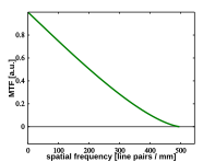
While it could be argued that the resolution of both the ideal and the imperfect system is 2 μm, or 500 LP/mm, it is clear that the images of the latter example are less sharp. A definition of resolution that is more in line with the perceived quality would instead use the spatial frequency at
565:
The impulse response of a well-focused optical system is a three-dimensional intensity distribution with a maximum at the focal plane, and could thus be measured by recording a stack of images while displacing the detector axially. By consequence, the three-dimensional optical transfer function can
3563:
line scanners were developed, which sampled more pixels than were needed and then downconverted, which is why movies have always looked sharper on television than other material shot with a video camera. The only theoretically correct way to interpolate or downconvert is by use of a steep low-pass
2566:
At high numerical apertures such as those found in microscopy, it is important to consider the vectorial nature of the fields that carry light. By decomposing the waves in three independent components corresponding to the
Cartesian axes, a point spread function can be calculated for each component
749:
It can be read from the plot that the contrast gradually reduces and reaches zero at the spatial frequency of 500 cycles per millimeter, in other words the optical resolution of the image projection is 1/500 of a millimeter, or 2 micrometer. Correspondingly, for this particular imaging device, the
903:
The three-dimensional point spread functions (a,c) and corresponding modulation transfer functions (b,d) of a wide-field microscope (a,b) and confocal microscope (c,d). In both cases the numerical aperture of the objective is 1.49 and the refractive index of the medium 1.52. The wavelength of the
3605:
Lens aperture diffraction also limits MTF. Whilst reducing the aperture of a lens usually reduces aberrations and hence improves the flatness of the MTF, there is an optimum aperture for any lens and image sensor size beyond which smaller apertures reduce resolution because of diffraction, which
3626:
effects. This has led to such cameras becoming preferred by some film and television program makers over even professional HD video cameras, because of their 'filmic' potential. In theory, the use of cameras with 16- and 21-megapixel sensors offers the possibility of almost perfect sharpness by
23:
Illustration of the optical transfer function (OTF) and its relation to image quality. The optical transfer function of a well-focused (a), and an out-of-focus optical imaging system without aberrations (d). As the optical transfer function of these systems is real and non-negative, the optical
3601:
Another factor in digital cameras and camcorders is lens resolution. A lens may be said to 'resolve' 1920 horizontal lines, but this does not mean that it does so with full modulation from black to white. The 'modulation transfer function' (just a term for the magnitude of the optical transfer
3587:
Just as standard definition video with a high contrast MTF is only possible with oversampling, so HD television with full theoretical sharpness is only possible by starting with a camera that has a significantly higher resolution, followed by digitally filtering. With movies now being shot in
2619:
When the aberrations can be assumed to be spatially invariant, alternative patterns can be used to determine the optical transfer function such as lines and edges. The corresponding transfer functions are referred to as the line-spread function and the edge-spread function, respectively. Such
881:
states that it should be possible, in a perfect system, to resolve fully (with true black to white transitions) a total of 1920 black and white alternating lines combined, otherwise referred to as a spatial frequency of 1920/2=960 line pairs per picture width, or 960 cycles per picture width,
844:
When viewed through an optical system with trefoil aberration, the image of a point object will look as a three-pointed star (a). As the point-spread function is not rotational symmetric, only a two-dimensional optical transfer function can describe it well (b). The height of the surface plot
900:
142:
Various closely related characterizations of an optical system exhibiting coma, a typical aberration that occurs off-axis. (a) The point-spread function (PSF) is the image of a point source. (b) The image of a line is referred to as the line-spread function, in this case a vertical line. The
908:
Although one typically thinks of an image as planar, or two-dimensional, the imaging system will produce a three-dimensional intensity distribution in image space that in principle can be measured. e.g. a two-dimensional sensor could be translated to capture a three-dimensional intensity
633:
should indicate the fraction of light that was detected from the point source object. However, typically the contrast relative to the total amount of detected light is most important. It is thus common practice to normalize the optical transfer function to the detected intensity, hence
2632:
The two-dimensional
Fourier transform of a line through the origin, is a line orthogonal to it and through the origin. The divisor is thus zero for all but a single dimension, by consequence, the optical transfer function can only be determined for a single dimension using a single
886:
will generally be reproduced with decreasing amplitude, so that fine detail, though it can be seen, is greatly reduced in contrast. This gives rise to the interesting observation that, for example, a standard definition television picture derived from a film scanner that uses
3181:
99:
of the optics, the image of a point source). As a
Fourier transform, the OTF is complex-valued; but it will be real-valued in the common case of a PSF that is symmetric about its center. The MTF is formally defined as the magnitude (absolute value) of the complex OTF.
3286:
2706:
3579:
function which requires powerful processing. In practice, various mathematical approximations to this are used to reduce the processing requirement. These approximations are now implemented widely in video editing systems and in image processing programs such as
2009:
862:
be seen that, while for the rotational symmetric aberrations the phase is either 0 or π and thus the transfer function is real valued, for the non-rotational symmetric aberration the transfer function has an imaginary component and the phase varies continuously.
1813:
1663:
3593:
image obtained from a 5-megapixel still camera can never be sharper than a 5-megapixel image obtained after down-conversion from an equal quality 10-megapixel still camera. Because of the problem of maintaining a high contrast MTF, broadcasters like the
1069:
The pupil function of an ideal optical system with a circular aperture is a disk of unit radius. The optical transfer function of such a system can thus be calculated geometrically from the intersecting area between two identical disks at a distance of
206:). Its values indicate how much of the object's contrast is captured in the image as a function of spatial frequency. The MTF tends to decrease with increasing spatial frequency from 1 to 0 (at the diffraction limit); however, the function is often not
882:(definitions in terms of cycles per unit angle or per mm are also possible but generally less clear when dealing with cameras and more appropriate to telescopes etc.). In practice, this is far from the case, and spatial frequencies that approach the
2640:
The line spread function can be found using two different methods. It can be found directly from an ideal line approximation provided by a slit test target or it can be derived from the edge spread function, discussed in the next sub section.
2553:
3530:
may not even be visible, and the finest patterns that can appear 'washed out' as shades of grey, not black and white. A major factor is usually the impossibility of making the perfect 'brick wall' optical filter (often realized as a
317:
197:
Often the contrast reduction is of most interest and the translation of the pattern can be ignored. The relative contrast is given by the absolute value of the optical transfer function, a function commonly referred to as the
396:
824:
spatial frequencies lower than 500 cycles per millimeter. This explains the gray circular bands in the spoke image shown in the above figure. In between the gray bands, the spokes appear to invert from black to white and
1019:
Mathematically both approaches are equivalent. Numeric calculations are typically most efficiently done via the
Fourier transform; however, analytic calculation may be more tractable using the auto-correlation approach.
3095:
480:
2620:
extended objects illuminate more pixels in the image, and can improve the measurement accuracy due to the larger signal-to-noise ratio. The optical transfer function is in this case calculated as the two-dimensional
832:
which the first zero occurs, 10 μm, or 100 LP/mm. Definitions of resolution, even for perfect imaging systems, vary widely. A more complete, unambiguous picture is provided by the optical transfer function.
828:, this is referred to as contrast inversion, directly related to the sign reversal in the real part of the optical transfer function, and represents itself as a shift by half a period for some periodic patterns.
3639:
of the display is reached. The optical contrast reduction can be partially reversed by digitally amplifying spatial frequencies selectively before display or further processing. Although more advanced digital
1383:
684:
Sometimes it is more practical to define the transfer functions based on a binary black-white stripe pattern. The transfer function for an equal-width black-white periodic pattern is referred to as the
1541:
3110:
2869:{\displaystyle \operatorname {ESF} ={\frac {X-\mu }{\sigma }}\qquad \qquad \sigma \,={\sqrt {\frac {\sum _{i=0}^{n-1}(x_{i}-\mu \,)^{2}}{n}}}\qquad \qquad \mu \,={\frac {\sum _{i=0}^{n-1}x_{i}}{n}}}
60:
specifies how different spatial frequencies are captured or transmitted. It is used by optical engineers to describe how the optics project light from the object or scene onto a photographic film,
3187:
1463:
631:
2336:
988:
has functionality to compute the optical or modulation transfer function of a lens design. Ideal systems such as in the examples here are readily calculated numerically using software such as
1854:
1721:
1549:
3478:
1218:
675:
1294:
753:
The resolution of a digital imaging device is not only limited by the optics, but also by the number of pixels, more in particular by their separation distance. As explained by the
520:
3363:
1846:
3506:
3448:
3420:
2224:
2259:
2166:
2070:
1703:
data versus spatial frequency is normalized by fitting a sixth order polynomial to it, making a smooth curve. The 50% cut-off frequency is determined and the corresponding
917:
that is half of that of the confocal microscope in all three-dimensions, confirming the previously noted lower resolution of the wide-field microscope. Note that along the
3610:) feature an "MTF autoexposure" mode, where the choice of aperture is optimized for maximum sharpness. Typically this means somewhere in the middle of the aperture range.
845:
indicates the absolute value and the hue indicates the complex argument of the function. A spoke target imaged by such an imaging device is shown by the simulation in (c).
2342:
3812:
Macias-Garza, F.; Bovik, A.; Diller, K.; Aggarwal, S.; Aggarwal, J. (1988). "The missing cone problem and low-pass distortion in optical serial sectioning microscopy".
3004:
3392:
2934:
2196:
2043:
1238:
3551:
The only way in practice to approach the theoretical sharpness possible in a digital imaging system such as a camera is to use more pixels in the camera sensor than
2981:
1137:
1091:
1157:
1111:
560:
540:
19:
3313:
3027:
2959:
2904:
2139:
2116:
2093:
1688:
curve to show the trend. The 50% cutoff frequency is determined to yield the corresponding spatial frequency. Thus, the approximate position of best focus of the
3559:
to avoid aliasing whilst maintaining a reasonably flat MTF up to that frequency. This approach was first taken in the 1970s when flying spot scanners, and later
2649:
The two-dimensional
Fourier transform of an edge is also only non-zero on a single line, orthogonal to the edge. This function is sometimes referred to as the
1113:
is the spatial frequency normalized to the highest transmitted frequency. In general the optical transfer function is normalized to a maximum value of one for
228:
103:
The image on the right shows the optical transfer functions for two different optical systems in panels (a) and (d). The former corresponds to the ideal,
328:
3698:
87:
pattern passing through the lens system, as a function of its spatial frequency or period, and its orientation. Formally, the OTF is defined as the
32:
are shown in (b,e) and (c,f), respectively. Note that the scale of the point source images (b,e) is four times smaller than the spoke target images.
817:
Transfer function and example image of an f/4 optical imaging system at 500 nm with spherical aberration with standard
Zernike coefficient of 0.25.
711:
optical imaging system used, at the visible wavelength of 500 nm, would have the optical transfer function depicted in the right hand figure.
3047:
402:
2637:(LSF). If necessary, the two-dimensional optical transfer function can be determined by repeating the measurement with lines at various angles.
936:
The two-dimensional optical transfer function at the focal plane can be calculated by integration of the 3D optical transfer function along the
3602:
function with phase ignored) gives the true measure of lens performance, and is represented by a graph of amplitude against spatial frequency.
2583:
The optical transfer function is not only useful for the design of optical system, it is also valuable to characterize manufactured systems.
123:
Since the optical transfer function (OTF) is defined as the
Fourier transform of the point-spread function (PSF), it is generally speaking a
3636:
878:
754:
3963:
3526:
In practice, many factors result in considerable blurring of a reproduced image, such that patterns with spatial frequency just below the
2603:. The optical transfer function is thus readily obtained by first acquiring the image of a point source, and applying the two-dimensional
731:
2607:
to the sampled image. Such a point-source can, for example, be a bright light behind a screen with a pin hole, a fluorescent or metallic
725:
The one-dimensional optical transfer function of a diffraction limited imaging system is identical to its modulation transfer function.
3857:
3775:
3619:
1299:
681:
When significant variation occurs, the optical transfer function may be calculated for a set of representative positions or colors.
3555:
in the final image, and 'downconvert' or 'interpolate' using special digital processing which cuts off high frequencies above the
3176:{\displaystyle \operatorname {LSF} ={\frac {d}{dx}}\operatorname {ESF} (x)\approx {\frac {\Delta \operatorname {ESF} }{\Delta x}}}
2558:
The MTF is then plotted against spatial frequency and all relevant data concerning this test can be determined from that graph.
1468:
4006:
793:
781:
3535:' or a lens with specific blurring properties in digital cameras and video camcorders). Such a filter is necessary to reduce
3281:{\displaystyle \operatorname {LSF} \approx {\frac {\operatorname {ESF} _{i+1}-\operatorname {ESF} _{i-1}}{2(x_{i+1}-x_{i})}}}
3041:. In case it is more practical to measure the edge spread function, one can determine the line spread function as follows:
719:
3992:
Mazzetta, J.A.; Scopatz, S.D. (2007). Automated Testing of Ultraviolet, Visible, and Infrared Sensors Using Shared Optics.
1388:
1000:, and in some specific cases even analytically. The optical transfer function can be calculated following two approaches:
854:
shows the two-dimensional equivalent of the ideal and the imperfect system discussed earlier, for an optical system with
576:
3552:
2267:
2004:{\displaystyle \operatorname {MTF} ={\mathcal {DFT}}=Y_{k}=\sum _{n=0}^{N-1}y_{n}e^{-ik{\frac {2\pi }{N}}n}\qquad k\in }
989:
1808:{\displaystyle \operatorname {MTF} ={\mathcal {F}}\left\qquad \qquad \operatorname {MTF} =\int f(x)e^{-i2\pi \,xs}\,dx}
1715:
The Fourier transform of the line spread function (LSF) can not be determined analytically by the following equations:
562:
is a vector with a spatial frequency for each dimension, i.e. it indicates also the direction of the periodic pattern.
3693:
805:
1658:{\displaystyle \operatorname {OTF} (\nu )={\frac {2}{\pi }}\left(\arccos(|\nu |)-|\nu |{\sqrt {1-\nu ^{2}}}\right).}
840:
2697:
2621:
2604:
1677:
104:
24:
transfer function is by definition equal to the modulation transfer function (MTF). Images of a point source and a
222:). The complex-valued optical transfer function can be seen as a combination of these two real-valued functions:
3455:
2624:
of the image and divided by that of the extended object. Typically either a line or a black-white edge is used.
3713:
3641:
1169:
637:
214:
of the optical transfer function can be depicted as a second real-valued function, commonly referred to as the
743:
Transfer function and example image of an ideal, optical-aberration-free (diffraction-limited) imaging system.
4040:
3886:
1243:
488:
131:. The projection of a specific periodic pattern is represented by a complex number with absolute value and
3747:
The exact definition of resolution may vary and is often taken to be 1.22 times larger as defined by the
3708:
3658:
3560:
2600:
1043:
1005:
914:
92:
4034:
3318:
1821:
956: = 0. This is only possible because the 3D optical transfer function diverges at the origin
3924:
3645:
3483:
3425:
3397:
3100:
Typically the ESF is only known at discrete points, so the LSF is numerically approximated using the
2201:
973:
2231:
2548:{\displaystyle \operatorname {MTF} ={\mathcal {DFT}}=Y_{k}=\sum _{n=0}^{N-1}y_{n}\left\qquad k\in }
2144:
2048:
1055:
985:
855:
850:
1818:
Therefore, the Fourier Transform is numerically approximated using the discrete Fourier transform
899:
3825:
3748:
3703:
3532:
3038:
877:
Taking the example of a current high definition (HD) video system, with 1920 by 1080 pixels, the
871:
770:
704:
135:
proportional to the relative contrast and translation of the projected projection, respectively.
3971:
2988:
138:
3853:
3771:
3723:
3101:
2592:
1681:
1039:
570:
128:
88:
80:
29:
3369:
2911:
2676:
As shown in the right hand figure, an operator defines a box area encompassing the edge of a
2173:
2020:
1223:
773:
imaging system could possess the optical transfer function depicted in the following figure.
3932:
3817:
3728:
3688:
3666:
2965:
2596:
1163:
1116:
211:
132:
96:
3791:
1073:
16:
Function that specifies how different spatial frequencies are captured by an optical system
4056:
1142:
1096:
1059:
1046:, and the point spread function is the square absolute of the inverse Fourier transformed
545:
525:
57:
3297:
3011:
2943:
2888:
2123:
2100:
2077:
940:-axis. Although the 3D transfer function of the wide-field microscope (b) is zero on the
787:
The real part of the optical transfer function of an aberrated, imperfect imaging system.
3928:
933:
is a well-known problem that prevents optical sectioning using a wide-field microscope.
3623:
1063:
1051:
1047:
1012:
124:
108:
3936:
3635:
Due to optical effects the contrast may be sub-optimal and approaches zero before the
2656:
4050:
3829:
3670:
3589:
2684:. The box area is defined to be approximately 10% of the total frame area. The image
312:{\displaystyle \mathrm {OTF} (\nu )=\mathrm {MTF} (\nu )e^{i\,\mathrm {PhTF} (\nu )}}
929: = 0, the transfer function is zero everywhere except at the origin. This
68:, screen, or simply the next item in the optical transmission chain. A variant, the
3718:
3556:
3540:
3527:
2693:
888:
883:
112:
61:
25:
3994:
Infrared Imaging Systems: Design Analysis, Modeling, and Testing XVIII, Vol. 6543
3913:"A 3D vectorial optical transfer function suitable for arbitrary pupil functions"
1162:
The intersecting area can be calculated as the sum of the areas of two identical
391:{\displaystyle \mathrm {MTF} (\nu )=\left\vert \mathrm {OTF} (\nu )\right\vert ,}
3814:
ICASSP-88., International Conference on Acoustics, Speech, and Signal Processing
3607:
3565:
2664:, an operator defines a box area equivalent to 10% of the total frame area of a
2608:
1695:
3912:
3821:
3662:
3034:
2681:
993:
49:
948: ≠ 0; its integral, the 2D optical transfer, reaching a maximum at
3581:
3576:
799:
The modulation transfer function of an aberrated, imperfect, imaging system.
207:
84:
76:), neglects phase effects, but is equivalent to the OTF in many situations.
53:
3090:{\displaystyle \operatorname {LSF} ={\frac {d}{dx}}\operatorname {ESF} (x)}
475:{\displaystyle \mathrm {PhTF} (\nu )=\mathrm {arg} (\mathrm {OTF} (\nu )),}
3874:
Numerical Methods for Engineers (5th ed.). New York, New York: McGraw-Hill
3547:
Oversampling and downconversion to maintain the optical transfer function
3536:
1050:, the optical transfer function can also be calculated directly from the
758:
708:
210:. On the other hand, when also the pattern translation is important, the
2692:
intensity and pixel position). The amplitude (pixel intensity) of each
1676:
The one-dimensional optical transfer function can be calculated as the
836:
The OTF of an optical system with a non-rotational symmetric aberration
3618:
There has recently been a shift towards the use of large image format
997:
811:
The image of a spoke target as imaged by an aberrated optical system.
65:
45:
2575:
optical transfer function can be determined as shown in () and ().
3683:
3661:, the image of a point source also depends on factors such as the
2689:
2685:
2655:
1694:
898:
839:
137:
18:
1058:
it can be seen that the optical transfer function is in fact the
2672:. The area is defined to encompass the edge of the target image.
3594:
1684:
data. In this case, a sixth order polynomial is fitted to the
1680:
of the line spread function. This data is graphed against the
1543:. Hence the normalized optical transfer function is given by:
1378:{\displaystyle \sin(\theta )/2=\sin(\theta /2)\cos(\theta /2)}
542:
is the spatial frequency of the periodic pattern. In general
3887:"Vectorial pupil functions and vectorial transfer functions"
3770:. SPIE – The International Society for Optical Engineering.
2360:
2357:
2354:
1872:
1869:
1866:
1833:
1830:
1827:
1733:
972:-axis of the 3D optical transfer function correspond to the
737:
Spoke target imaged by a diffraction limited imaging system.
3037:
of the edge spread function, which is differentiated using
2615:
Using extended test objects for spatially invariant optics
1536:{\displaystyle \arccos(|\nu |)-|\nu |{\sqrt {1-\nu ^{2}}}}
2883:
ESF = the output array of normalized pixel intensity data
3622:
driven by the need for low-light sensitivity and narrow
761:
may lead to a further reduction of the image fidelity.
3614:
Trend to large-format DSLRs and improved MTF potential
3486:
3458:
3428:
3400:
3372:
3321:
3300:
3190:
3113:
3050:
3014:
2991:
2968:
2946:
2914:
2891:
2709:
2345:
2270:
2234:
2204:
2176:
2147:
2126:
2103:
2080:
2051:
2023:
1857:
1824:
1724:
1552:
1471:
1391:
1302:
1246:
1226:
1172:
1145:
1119:
1099:
1076:
640:
579:
548:
528:
491:
405:
331:
231:
3006:= the standard deviation of the pixel intensity data
2700:
and averaged. This yields the edge spread function.
1458:{\displaystyle 1=\nu ^{2}+\sin(\arccos(|\nu |))^{2}}
4041:"How to Measure MTF and other Properties of Lenses"
3953:(2nd ed.). Florida:JCD Publishing, Washington:SPIE.
626:{\displaystyle \mathrm {OTF} (0)=\mathrm {MTF} (0)}
3951:Testing and Evaluation of Infrared Imaging Systems
3500:
3472:
3442:
3414:
3386:
3357:
3307:
3280:
3175:
3089:
3021:
2998:
2975:
2953:
2928:
2898:
2868:
2547:
2331:{\displaystyle e^{\pm ia}=\cos(a)\,\pm \,i\sin(a)}
2330:
2253:
2218:
2190:
2160:
2133:
2110:
2087:
2064:
2037:
2003:
1840:
1807:
1657:
1535:
1457:
1377:
1288:
1232:
1212:
1151:
1131:
1105:
1085:
669:
625:
554:
534:
514:
474:
390:
311:
2688:data is translated into a two-dimensional array (
1668:A more detailed discussion can be found in and.
2591:The optical transfer function is defined as the
1465:, the equation for the area can be rewritten as
866:Practical example – high-definition video system
522:represents the complex argument function, while
3522:Factors affecting MTF in typical camera systems
2983:= the average value of the pixel intensity data
1707:is found, yielding the approximate position of
895:The three-dimensional optical transfer function
3761:
3759:
3757:
968: = 0. The function values along the
3852:(3rd ed.). Roberts & Co Publishers.
3843:
3841:
3839:
3768:Introduction to the Optical Transfer Function
3539:by eliminating spatial frequencies above the
3033:The line spread function is identical to the
1240:is the circle segment angle. By substituting
1139:, so the resulting area should be divided by
8:
913:function of the wide-field microscope has a
3911:Arnison, M. R.; Sheppard, C. J. R. (2002).
1038:Since the optical transfer function is the
1004:as the Fourier transform of the incoherent
169:1D section of 2D optical-transfer function
3473:{\displaystyle \operatorname {ESF} _{i}\,}
146:
3699:Minimum resolvable temperature difference
3497:
3491:
3485:
3469:
3463:
3457:
3439:
3433:
3427:
3411:
3405:
3399:
3383:
3377:
3371:
3320:
3304:
3299:
3266:
3247:
3223:
3204:
3197:
3189:
3153:
3120:
3112:
3057:
3049:
3018:
3013:
2995:
2990:
2972:
2967:
2950:
2945:
2925:
2919:
2913:
2906:= the input array of pixel intensity data
2895:
2890:
2854:
2838:
2827:
2820:
2816:
2798:
2793:
2781:
2762:
2751:
2743:
2739:
2716:
2708:
2489:
2446:
2421:
2405:
2394:
2381:
2353:
2352:
2344:
2309:
2305:
2275:
2269:
2241:
2233:
2215:
2209:
2203:
2187:
2181:
2175:
2152:
2146:
2130:
2125:
2107:
2102:
2084:
2079:
2056:
2050:
2034:
2028:
2022:
1953:
1943:
1933:
1917:
1906:
1893:
1865:
1864:
1856:
1826:
1825:
1823:
1798:
1789:
1776:
1732:
1731:
1723:
1639:
1627:
1622:
1614:
1603:
1595:
1571:
1551:
1525:
1513:
1508:
1500:
1489:
1481:
1470:
1449:
1437:
1429:
1402:
1390:
1364:
1341:
1318:
1301:
1275:
1255:
1247:
1245:
1225:
1213:{\displaystyle \theta /2-\sin(\theta )/2}
1202:
1176:
1171:
1144:
1118:
1098:
1075:
858:, a non-rotational-symmetric aberration.
670:{\displaystyle \mathrm {MTF} (0)\equiv 1}
641:
639:
603:
580:
578:
547:
527:
492:
490:
446:
432:
406:
404:
360:
332:
330:
284:
283:
279:
255:
232:
230:
4037:, by Glenn D. Boreman on SPIE Optipedia.
4007:"B2BVideoSource.com: Camera Terminology"
1029:Ideal lens system with circular aperture
3964:"Test and Measurement – Products – EOI"
3740:
2599:of the optical system, also called the
2587:Starting from the point spread function
1289:{\displaystyle |\nu |=\cos(\theta /2)}
1034:Auto-correlation of the pupil function
515:{\displaystyle \mathrm {arg} (\cdot )}
3885:Sheppard, C.J.R.; Larkin, K. (1997).
3513:Using a grid of black and white lines
166:(derivative of edge-spread function)
83:specifies the response to a periodic
7:
2571:point spread function. Similarly, a
3872:Chapra, S.C.; Canale, R.P. (2006).
849:Optical systems, and in particular
3620:digital single-lens reflex cameras
3164:
3156:
3029:= number of pixels used in average
648:
645:
642:
610:
607:
604:
587:
584:
581:
499:
496:
493:
453:
450:
447:
439:
436:
433:
416:
413:
410:
407:
367:
364:
361:
339:
336:
333:
294:
291:
288:
285:
262:
259:
256:
239:
236:
233:
14:
3816:. Vol. 2. pp. 890–893.
107:, imaging system with a circular
44:) of an optical system such as a
3358:{\displaystyle i=1,2,\dots ,n-1}
1841:{\displaystyle {\mathcal {DFT}}}
804:
792:
780:
755:Nyquist–Shannon sampling theorem
730:
718:
687:contrast transfer function (CTF)
3674:the optical system accurately.
3501:{\displaystyle i^{\text{th}}\,}
3443:{\displaystyle i^{\text{th}}\,}
3415:{\displaystyle i^{\text{th}}\,}
2812:
2811:
2735:
2734:
2562:The vectorial transfer function
2517:
2219:{\displaystyle n^{\text{th}}\,}
1973:
1750:
1749:
1011:as the auto-correlation of the
765:OTF of an imperfect lens system
698:The OTF of an ideal lens system
180:(2D) Optical transfer function
119:Definition and related concepts
4035:"Modulation transfer function"
3850:Introduction to Fourier Optics
3272:
3240:
3147:
3141:
3084:
3078:
2795:
2774:
2542:
2524:
2371:
2365:
2325:
2319:
2302:
2296:
2254:{\displaystyle i={\sqrt {-1}}}
1998:
1980:
1883:
1877:
1769:
1763:
1692:is determined from this data.
1623:
1615:
1608:
1604:
1596:
1592:
1565:
1559:
1509:
1501:
1494:
1490:
1482:
1478:
1446:
1442:
1438:
1430:
1426:
1417:
1372:
1358:
1349:
1335:
1315:
1309:
1283:
1269:
1256:
1248:
1199:
1193:
658:
652:
620:
614:
597:
591:
509:
503:
466:
463:
457:
443:
426:
420:
377:
371:
349:
343:
304:
298:
272:
266:
249:
243:
1:
3937:10.1016/S0030-4018(02)01857-6
3766:Williams, Charles S. (2002).
2161:{\displaystyle k^{\text{th}}}
2065:{\displaystyle k^{\text{th}}}
191:3D Optical-transfer function
3792:"Contrast Transfer Function"
3631:Digital inversion of the OTF
3564:spatial filter, realized by
2680:image back-illuminated by a
200:modulation transfer function
70:modulation transfer function
3694:Minimum resolvable contrast
3568:with a two-dimensional sin(
1296:, and using the equalities
4073:
3822:10.1109/ICASSP.1988.196731
2622:discrete Fourier transform
2605:discrete Fourier transform
1678:discrete Fourier transform
569:True to the definition of
4043:, by Optikos Corporation.
2999:{\displaystyle \sigma \,}
1686:MTF vs. spatial frequency
188:3D Point-spread function
38:optical transfer function
3996:, pp. 654313-1 654313-14
3848:Goodman, Joseph (2005).
3714:Signal transfer function
2628:The line-spread function
3968:www.Electro-Optical.com
3387:{\displaystyle x_{i}\,}
2929:{\displaystyle x_{i}\,}
2191:{\displaystyle y_{n}\,}
2095:= number of data points
2038:{\displaystyle Y_{k}\,}
1233:{\displaystyle \theta }
986:optical design software
216:phase transfer function
4011:www.B2BVideoSource.com
3644:procedures exist, the
3502:
3474:
3444:
3416:
3388:
3359:
3309:
3282:
3177:
3091:
3023:
3000:
2977:
2976:{\displaystyle \mu \,}
2955:
2930:
2900:
2870:
2849:
2773:
2678:knife-edge test target
2673:
2668:back-illuminated by a
2666:knife-edge test target
2549:
2416:
2332:
2255:
2220:
2192:
2162:
2135:
2112:
2089:
2066:
2039:
2005:
1928:
1842:
1809:
1712:
1659:
1537:
1459:
1379:
1290:
1234:
1214:
1153:
1133:
1132:{\displaystyle \nu =0}
1107:
1087:
905:
846:
671:
627:
556:
536:
516:
476:
392:
313:
177:Point-spread function
144:
33:
3917:Optics Communications
3709:Signal-to-noise ratio
3659:point spread function
3598:of true HD viewing).
3503:
3475:
3445:
3417:
3389:
3360:
3310:
3283:
3178:
3092:
3024:
3001:
2978:
2956:
2931:
2901:
2871:
2823:
2747:
2659:
2601:point spread function
2550:
2390:
2333:
2256:
2221:
2193:
2163:
2136:
2113:
2090:
2067:
2040:
2006:
1902:
1843:
1810:
1698:
1660:
1538:
1460:
1380:
1291:
1235:
1215:
1154:
1134:
1108:
1088:
1086:{\displaystyle 2\nu }
1044:point spread function
1015:of the optical system
1006:point spread function
902:
843:
672:
628:
557:
537:
517:
477:
393:
314:
141:
115:is relatively sharp.
93:point spread function
22:
3949:Holst, G.C. (1998).
3646:Wiener deconvolution
3484:
3456:
3426:
3398:
3370:
3319:
3298:
3188:
3111:
3048:
3012:
2989:
2966:
2944:
2912:
2889:
2707:
2696:within the array is
2651:edge spread function
2645:Edge-spread function
2635:line-spread function
2567:and combined into a
2343:
2268:
2232:
2202:
2174:
2168:term of the LSF data
2145:
2124:
2101:
2078:
2049:
2021:
1855:
1822:
1722:
1672:Numerical evaluation
1550:
1469:
1389:
1300:
1244:
1224:
1170:
1152:{\displaystyle \pi }
1143:
1117:
1106:{\displaystyle \nu }
1097:
1074:
974:Dirac delta function
703:example, a perfect,
638:
577:
555:{\displaystyle \nu }
546:
535:{\displaystyle \nu }
526:
489:
403:
329:
229:
164:Line-spread function
3929:2002OptCo.211...53A
3308:{\displaystyle i\,}
3022:{\displaystyle n\,}
2954:{\displaystyle X\,}
2899:{\displaystyle X\,}
2134:{\displaystyle k\,}
2111:{\displaystyle n\,}
2088:{\displaystyle N\,}
1056:convolution theorem
851:optical aberrations
105:diffraction-limited
95:(PSF, that is, the
3749:Rayleigh criterion
3704:Optical resolution
3498:
3470:
3440:
3412:
3384:
3355:
3305:
3278:
3173:
3087:
3019:
2996:
2973:
2951:
2926:
2896:
2866:
2674:
2660:In evaluating the
2545:
2328:
2251:
2216:
2188:
2158:
2131:
2108:
2085:
2062:
2035:
2001:
1838:
1805:
1713:
1655:
1533:
1455:
1375:
1286:
1230:
1210:
1149:
1129:
1103:
1083:
906:
872:optical resolution
847:
667:
623:
552:
532:
512:
472:
388:
309:
156:Fourier transform
145:
34:
3974:on 28 August 2008
3724:Transfer function
3642:image restoration
3637:Nyquist frequency
3494:
3436:
3408:
3276:
3171:
3133:
3102:finite difference
3070:
3039:numerical methods
2864:
2809:
2808:
2732:
2593:Fourier transform
2502:
2459:
2249:
2212:
2155:
2059:
1966:
1705:spatial frequency
1682:spatial frequency
1645:
1579:
1531:
1164:circular segments
1040:Fourier transform
571:transfer function
195:
194:
129:spatial frequency
89:Fourier transform
81:transfer function
30:spatial frequency
4064:
4022:
4021:
4019:
4017:
4003:
3997:
3990:
3984:
3983:
3981:
3979:
3970:. Archived from
3960:
3954:
3947:
3941:
3940:
3908:
3902:
3901:
3891:
3882:
3876:
3870:
3864:
3863:
3845:
3834:
3833:
3809:
3803:
3802:
3800:
3798:
3788:
3782:
3781:
3763:
3752:
3745:
3729:Wavefront coding
3689:Gamma correction
3657:In general, the
3543:of the display.
3507:
3505:
3504:
3499:
3496:
3495:
3492:
3479:
3477:
3476:
3471:
3468:
3467:
3449:
3447:
3446:
3441:
3438:
3437:
3434:
3422:position of the
3421:
3419:
3418:
3413:
3410:
3409:
3406:
3393:
3391:
3390:
3385:
3382:
3381:
3364:
3362:
3361:
3356:
3314:
3312:
3311:
3306:
3287:
3285:
3284:
3279:
3277:
3275:
3271:
3270:
3258:
3257:
3235:
3234:
3233:
3215:
3214:
3198:
3182:
3180:
3179:
3174:
3172:
3170:
3162:
3154:
3134:
3132:
3121:
3096:
3094:
3093:
3088:
3071:
3069:
3058:
3035:first derivative
3028:
3026:
3025:
3020:
3005:
3003:
3002:
2997:
2982:
2980:
2979:
2974:
2960:
2958:
2957:
2952:
2935:
2933:
2932:
2927:
2924:
2923:
2905:
2903:
2902:
2897:
2875:
2873:
2872:
2867:
2865:
2860:
2859:
2858:
2848:
2837:
2821:
2810:
2804:
2803:
2802:
2786:
2785:
2772:
2761:
2745:
2744:
2733:
2728:
2717:
2597:impulse response
2554:
2552:
2551:
2546:
2516:
2512:
2511:
2507:
2503:
2498:
2490:
2468:
2464:
2460:
2455:
2447:
2426:
2425:
2415:
2404:
2386:
2385:
2364:
2363:
2337:
2335:
2334:
2329:
2286:
2285:
2260:
2258:
2257:
2252:
2250:
2242:
2225:
2223:
2222:
2217:
2214:
2213:
2210:
2197:
2195:
2194:
2189:
2186:
2185:
2167:
2165:
2164:
2159:
2157:
2156:
2153:
2140:
2138:
2137:
2132:
2117:
2115:
2114:
2109:
2094:
2092:
2091:
2086:
2072:value of the MTF
2071:
2069:
2068:
2063:
2061:
2060:
2057:
2044:
2042:
2041:
2036:
2033:
2032:
2010:
2008:
2007:
2002:
1972:
1971:
1967:
1962:
1954:
1938:
1937:
1927:
1916:
1898:
1897:
1876:
1875:
1847:
1845:
1844:
1839:
1837:
1836:
1814:
1812:
1811:
1806:
1797:
1796:
1748:
1737:
1736:
1664:
1662:
1661:
1656:
1651:
1647:
1646:
1644:
1643:
1628:
1626:
1618:
1607:
1599:
1580:
1572:
1542:
1540:
1539:
1534:
1532:
1530:
1529:
1514:
1512:
1504:
1493:
1485:
1464:
1462:
1461:
1456:
1454:
1453:
1441:
1433:
1407:
1406:
1384:
1382:
1381:
1376:
1368:
1345:
1322:
1295:
1293:
1292:
1287:
1279:
1259:
1251:
1239:
1237:
1236:
1231:
1219:
1217:
1216:
1211:
1206:
1180:
1158:
1156:
1155:
1150:
1138:
1136:
1135:
1130:
1112:
1110:
1109:
1104:
1092:
1090:
1089:
1084:
808:
796:
784:
734:
722:
676:
674:
673:
668:
651:
632:
630:
629:
624:
613:
590:
561:
559:
558:
553:
541:
539:
538:
533:
521:
519:
518:
513:
502:
481:
479:
478:
473:
456:
442:
419:
397:
395:
394:
389:
384:
380:
370:
342:
318:
316:
315:
310:
308:
307:
297:
265:
242:
212:complex argument
153:Spatial function
147:
133:complex argument
97:impulse response
4072:
4071:
4067:
4066:
4065:
4063:
4062:
4061:
4047:
4046:
4031:
4026:
4025:
4015:
4013:
4005:
4004:
4000:
3991:
3987:
3977:
3975:
3962:
3961:
3957:
3948:
3944:
3910:
3909:
3905:
3894:Optik-Stuttgart
3889:
3884:
3883:
3879:
3871:
3867:
3860:
3847:
3846:
3837:
3811:
3810:
3806:
3796:
3794:
3790:
3789:
3785:
3778:
3765:
3764:
3755:
3746:
3742:
3737:
3680:
3655:
3633:
3616:
3549:
3524:
3515:
3487:
3482:
3481:
3459:
3454:
3453:
3429:
3424:
3423:
3401:
3396:
3395:
3373:
3368:
3367:
3317:
3316:
3296:
3295:
3262:
3243:
3236:
3219:
3200:
3199:
3186:
3185:
3163:
3155:
3125:
3109:
3108:
3062:
3046:
3045:
3010:
3009:
2987:
2986:
2964:
2963:
2942:
2941:
2915:
2910:
2909:
2887:
2886:
2850:
2822:
2794:
2777:
2746:
2718:
2705:
2704:
2647:
2630:
2617:
2589:
2581:
2564:
2491:
2485:
2481:
2448:
2442:
2438:
2431:
2427:
2417:
2377:
2341:
2340:
2271:
2266:
2265:
2230:
2229:
2205:
2200:
2199:
2177:
2172:
2171:
2148:
2143:
2142:
2122:
2121:
2099:
2098:
2076:
2075:
2052:
2047:
2046:
2024:
2019:
2018:
1955:
1939:
1929:
1889:
1853:
1852:
1820:
1819:
1772:
1738:
1720:
1719:
1690:unit under test
1674:
1635:
1585:
1581:
1548:
1547:
1521:
1467:
1466:
1445:
1398:
1387:
1386:
1298:
1297:
1242:
1241:
1222:
1221:
1168:
1167:
1141:
1140:
1115:
1114:
1095:
1094:
1072:
1071:
1060:autocorrelation
1036:
1031:
1026:
982:
897:
879:Nyquist theorem
868:
838:
821:
820:
819:
818:
814:
813:
812:
809:
801:
800:
797:
789:
788:
785:
767:
747:
746:
745:
744:
740:
739:
738:
735:
727:
726:
723:
700:
695:
636:
635:
575:
574:
544:
543:
524:
523:
487:
486:
401:
400:
359:
355:
327:
326:
275:
227:
226:
165:
121:
17:
12:
11:
5:
4070:
4068:
4060:
4059:
4049:
4048:
4045:
4044:
4038:
4030:
4029:External links
4027:
4024:
4023:
3998:
3985:
3955:
3942:
3923:(1–6): 53–63.
3903:
3877:
3865:
3858:
3835:
3804:
3783:
3776:
3753:
3739:
3738:
3736:
3733:
3732:
3731:
3726:
3721:
3716:
3711:
3706:
3701:
3696:
3691:
3686:
3679:
3676:
3654:
3651:
3632:
3629:
3624:depth of field
3615:
3612:
3548:
3545:
3523:
3520:
3514:
3511:
3510:
3509:
3490:
3466:
3462:
3451:
3432:
3404:
3380:
3376:
3365:
3354:
3351:
3348:
3345:
3342:
3339:
3336:
3333:
3330:
3327:
3324:
3303:
3289:
3288:
3274:
3269:
3265:
3261:
3256:
3253:
3250:
3246:
3242:
3239:
3232:
3229:
3226:
3222:
3218:
3213:
3210:
3207:
3203:
3196:
3193:
3183:
3169:
3166:
3161:
3158:
3152:
3149:
3146:
3143:
3140:
3137:
3131:
3128:
3124:
3119:
3116:
3098:
3097:
3086:
3083:
3080:
3077:
3074:
3068:
3065:
3061:
3056:
3053:
3031:
3030:
3017:
3007:
2994:
2984:
2971:
2961:
2949:
2922:
2918:
2907:
2894:
2884:
2877:
2876:
2863:
2857:
2853:
2847:
2844:
2841:
2836:
2833:
2830:
2826:
2819:
2815:
2807:
2801:
2797:
2792:
2789:
2784:
2780:
2776:
2771:
2768:
2765:
2760:
2757:
2754:
2750:
2742:
2738:
2731:
2727:
2724:
2721:
2715:
2712:
2646:
2643:
2629:
2626:
2616:
2613:
2588:
2585:
2580:
2577:
2563:
2560:
2556:
2555:
2544:
2541:
2538:
2535:
2532:
2529:
2526:
2523:
2520:
2515:
2510:
2506:
2501:
2497:
2494:
2488:
2484:
2480:
2477:
2474:
2471:
2467:
2463:
2458:
2454:
2451:
2445:
2441:
2437:
2434:
2430:
2424:
2420:
2414:
2411:
2408:
2403:
2400:
2397:
2393:
2389:
2384:
2380:
2376:
2373:
2370:
2367:
2362:
2359:
2356:
2351:
2348:
2338:
2327:
2324:
2321:
2318:
2315:
2312:
2308:
2304:
2301:
2298:
2295:
2292:
2289:
2284:
2281:
2278:
2274:
2262:
2261:
2248:
2245:
2240:
2237:
2227:
2226:pixel position
2208:
2184:
2180:
2169:
2151:
2129:
2119:
2106:
2096:
2083:
2073:
2055:
2031:
2027:
2012:
2011:
2000:
1997:
1994:
1991:
1988:
1985:
1982:
1979:
1976:
1970:
1965:
1961:
1958:
1952:
1949:
1946:
1942:
1936:
1932:
1926:
1923:
1920:
1915:
1912:
1909:
1905:
1901:
1896:
1892:
1888:
1885:
1882:
1879:
1874:
1871:
1868:
1863:
1860:
1835:
1832:
1829:
1816:
1815:
1804:
1801:
1795:
1792:
1788:
1785:
1782:
1779:
1775:
1771:
1768:
1765:
1762:
1759:
1756:
1753:
1747:
1744:
1741:
1735:
1730:
1727:
1673:
1670:
1666:
1665:
1654:
1650:
1642:
1638:
1634:
1631:
1625:
1621:
1617:
1613:
1610:
1606:
1602:
1598:
1594:
1591:
1588:
1584:
1578:
1575:
1570:
1567:
1564:
1561:
1558:
1555:
1528:
1524:
1520:
1517:
1511:
1507:
1503:
1499:
1496:
1492:
1488:
1484:
1480:
1477:
1474:
1452:
1448:
1444:
1440:
1436:
1432:
1428:
1425:
1422:
1419:
1416:
1413:
1410:
1405:
1401:
1397:
1394:
1374:
1371:
1367:
1363:
1360:
1357:
1354:
1351:
1348:
1344:
1340:
1337:
1334:
1331:
1328:
1325:
1321:
1317:
1314:
1311:
1308:
1305:
1285:
1282:
1278:
1274:
1271:
1268:
1265:
1262:
1258:
1254:
1250:
1229:
1209:
1205:
1201:
1198:
1195:
1192:
1189:
1186:
1183:
1179:
1175:
1148:
1128:
1125:
1122:
1102:
1082:
1079:
1064:pupil function
1052:pupil function
1048:pupil function
1035:
1032:
1030:
1027:
1025:
1022:
1017:
1016:
1013:pupil function
1009:
981:
978:
896:
893:
867:
864:
837:
834:
816:
815:
810:
803:
802:
798:
791:
790:
786:
779:
778:
777:
776:
775:
769:An imperfect,
766:
763:
742:
741:
736:
729:
728:
724:
717:
716:
715:
714:
713:
699:
696:
694:
691:
666:
663:
660:
657:
654:
650:
647:
644:
622:
619:
616:
612:
609:
606:
602:
599:
596:
593:
589:
586:
583:
551:
531:
511:
508:
505:
501:
498:
495:
483:
482:
471:
468:
465:
462:
459:
455:
452:
449:
445:
441:
438:
435:
431:
428:
425:
422:
418:
415:
412:
409:
398:
387:
383:
379:
376:
373:
369:
366:
363:
358:
354:
351:
348:
345:
341:
338:
335:
320:
319:
306:
303:
300:
296:
293:
290:
287:
282:
278:
274:
271:
268:
264:
261:
258:
254:
251:
248:
245:
241:
238:
235:
193:
192:
189:
186:
182:
181:
178:
175:
171:
170:
167:
162:
158:
157:
154:
151:
125:complex-valued
120:
117:
62:detector array
15:
13:
10:
9:
6:
4:
3:
2:
4069:
4058:
4055:
4054:
4052:
4042:
4039:
4036:
4033:
4032:
4028:
4012:
4008:
4002:
3999:
3995:
3989:
3986:
3973:
3969:
3965:
3959:
3956:
3952:
3946:
3943:
3938:
3934:
3930:
3926:
3922:
3918:
3914:
3907:
3904:
3899:
3895:
3888:
3881:
3878:
3875:
3869:
3866:
3861:
3859:0-9747077-2-4
3855:
3851:
3844:
3842:
3840:
3836:
3831:
3827:
3823:
3819:
3815:
3808:
3805:
3793:
3787:
3784:
3779:
3777:0-8194-4336-0
3773:
3769:
3762:
3760:
3758:
3754:
3750:
3744:
3741:
3734:
3730:
3727:
3725:
3722:
3720:
3717:
3715:
3712:
3710:
3707:
3705:
3702:
3700:
3697:
3695:
3692:
3690:
3687:
3685:
3682:
3681:
3677:
3675:
3672:
3668:
3664:
3660:
3652:
3650:
3647:
3643:
3638:
3630:
3628:
3625:
3621:
3613:
3611:
3609:
3603:
3599:
3596:
3591:
3585:
3583:
3578:
3575:
3571:
3567:
3562:
3558:
3554:
3546:
3544:
3542:
3538:
3534:
3529:
3521:
3519:
3512:
3488:
3480:= ESF of the
3464:
3460:
3452:
3430:
3402:
3378:
3374:
3366:
3352:
3349:
3346:
3343:
3340:
3337:
3334:
3331:
3328:
3325:
3322:
3301:
3294:
3293:
3292:
3267:
3263:
3259:
3254:
3251:
3248:
3244:
3237:
3230:
3227:
3224:
3220:
3216:
3211:
3208:
3205:
3201:
3194:
3191:
3184:
3167:
3159:
3150:
3144:
3138:
3135:
3129:
3126:
3122:
3117:
3114:
3107:
3106:
3105:
3103:
3081:
3075:
3072:
3066:
3063:
3059:
3054:
3051:
3044:
3043:
3042:
3040:
3036:
3015:
3008:
2992:
2985:
2969:
2962:
2947:
2939:
2920:
2916:
2908:
2892:
2885:
2882:
2881:
2880:
2861:
2855:
2851:
2845:
2842:
2839:
2834:
2831:
2828:
2824:
2817:
2813:
2805:
2799:
2790:
2787:
2782:
2778:
2769:
2766:
2763:
2758:
2755:
2752:
2748:
2740:
2736:
2729:
2725:
2722:
2719:
2713:
2710:
2703:
2702:
2701:
2699:
2695:
2691:
2687:
2683:
2679:
2671:
2667:
2663:
2658:
2654:
2652:
2644:
2642:
2638:
2636:
2627:
2625:
2623:
2614:
2612:
2610:
2606:
2602:
2598:
2594:
2586:
2584:
2578:
2576:
2574:
2570:
2561:
2559:
2539:
2536:
2533:
2530:
2527:
2521:
2518:
2513:
2508:
2504:
2499:
2495:
2492:
2486:
2482:
2478:
2475:
2472:
2469:
2465:
2461:
2456:
2452:
2449:
2443:
2439:
2435:
2432:
2428:
2422:
2418:
2412:
2409:
2406:
2401:
2398:
2395:
2391:
2387:
2382:
2378:
2374:
2368:
2349:
2346:
2339:
2322:
2316:
2313:
2310:
2306:
2299:
2293:
2290:
2287:
2282:
2279:
2276:
2272:
2264:
2263:
2246:
2243:
2238:
2235:
2228:
2206:
2182:
2178:
2170:
2149:
2127:
2120:
2104:
2097:
2081:
2074:
2053:
2029:
2025:
2017:
2016:
2015:
1995:
1992:
1989:
1986:
1983:
1977:
1974:
1968:
1963:
1959:
1956:
1950:
1947:
1944:
1940:
1934:
1930:
1924:
1921:
1918:
1913:
1910:
1907:
1903:
1899:
1894:
1890:
1886:
1880:
1861:
1858:
1851:
1850:
1849:
1802:
1799:
1793:
1790:
1786:
1783:
1780:
1777:
1773:
1766:
1760:
1757:
1754:
1751:
1745:
1742:
1739:
1728:
1725:
1718:
1717:
1716:
1710:
1706:
1702:
1697:
1693:
1691:
1687:
1683:
1679:
1671:
1669:
1652:
1648:
1640:
1636:
1632:
1629:
1619:
1611:
1600:
1589:
1586:
1582:
1576:
1573:
1568:
1562:
1556:
1553:
1546:
1545:
1544:
1526:
1522:
1518:
1515:
1505:
1497:
1486:
1475:
1472:
1450:
1434:
1423:
1420:
1414:
1411:
1408:
1403:
1399:
1395:
1392:
1369:
1365:
1361:
1355:
1352:
1346:
1342:
1338:
1332:
1329:
1326:
1323:
1319:
1312:
1306:
1303:
1280:
1276:
1272:
1266:
1263:
1260:
1252:
1227:
1207:
1203:
1196:
1190:
1187:
1184:
1181:
1177:
1173:
1165:
1160:
1146:
1126:
1123:
1120:
1100:
1080:
1077:
1067:
1065:
1061:
1057:
1053:
1049:
1045:
1041:
1033:
1028:
1023:
1021:
1014:
1010:
1007:
1003:
1002:
1001:
999:
995:
991:
987:
979:
977:
975:
971:
967:
964: =
963:
960: =
959:
955:
952: =
951:
947:
943:
939:
934:
932:
928:
925: =
924:
920:
916:
910:
901:
894:
892:
890:
885:
880:
875:
873:
865:
863:
859:
857:
852:
842:
835:
833:
829:
827:
807:
795:
783:
774:
772:
764:
762:
760:
756:
751:
733:
721:
712:
710:
706:
705:non-aberrated
697:
692:
690:
688:
682:
678:
664:
661:
655:
617:
600:
594:
572:
567:
563:
549:
529:
506:
469:
460:
429:
423:
399:
385:
381:
374:
356:
352:
346:
325:
324:
323:
301:
280:
276:
269:
252:
246:
225:
224:
223:
221:
217:
213:
209:
205:
201:
190:
187:
184:
183:
179:
176:
173:
172:
168:
163:
160:
159:
155:
152:
149:
148:
140:
136:
134:
130:
126:
118:
116:
114:
110:
106:
101:
98:
94:
90:
86:
82:
77:
75:
71:
67:
63:
59:
55:
51:
47:
43:
39:
31:
27:
21:
4014:. Retrieved
4010:
4001:
3993:
3988:
3976:. Retrieved
3972:the original
3967:
3958:
3950:
3945:
3920:
3916:
3906:
3897:
3893:
3880:
3873:
3868:
3849:
3813:
3807:
3795:. Retrieved
3786:
3767:
3743:
3719:Strehl ratio
3656:
3634:
3617:
3604:
3600:
3586:
3573:
3569:
3557:Nyquist rate
3550:
3541:Nyquist rate
3528:Nyquist rate
3525:
3516:
3315:= the index
3290:
3099:
3032:
2937:
2878:
2677:
2675:
2669:
2665:
2661:
2650:
2648:
2639:
2634:
2631:
2618:
2590:
2582:
2572:
2568:
2565:
2557:
2013:
1817:
1714:
1708:
1704:
1700:
1689:
1685:
1675:
1667:
1161:
1068:
1037:
1018:
983:
969:
965:
961:
957:
953:
949:
945:
941:
937:
935:
931:missing cone
930:
926:
922:
918:
911:
907:
889:oversampling
884:Nyquist rate
876:
869:
860:
848:
830:
825:
822:
768:
752:
748:
701:
686:
683:
679:
568:
564:
484:
321:
219:
215:
203:
199:
196:
127:function of
122:
113:spoke target
102:
78:
73:
69:
41:
37:
35:
26:spoke target
3797:16 November
3653:Limitations
3608:Pentax K10D
3566:convolution
3533:phase plate
2940:element of
2609:microsphere
2579:Measurement
1054:. From the
980:Calculation
921:-axis, for
3735:References
3663:wavelength
2698:normalized
2682:black body
2670:black body
1709:best focus
994:GNU Octave
944:-axis for
826:vice versa
150:Dimensions
50:microscope
28:with high
4016:2 January
3978:2 January
3830:120191405
3582:Photoshop
3577:weighting
3350:−
3341:…
3260:−
3228:−
3217:−
3195:≈
3165:Δ
3157:Δ
3151:≈
3139:
3076:
2993:σ
2970:μ
2843:−
2825:∑
2814:μ
2791:μ
2788:−
2767:−
2749:∑
2737:σ
2730:σ
2726:μ
2723:−
2573:vectorial
2569:vectorial
2537:−
2522:∈
2496:π
2479:
2470:−
2453:π
2436:
2410:−
2392:∑
2317:
2307:±
2294:
2277:±
2244:−
1993:−
1978:∈
1960:π
1945:−
1922:−
1904:∑
1787:π
1778:−
1758:∫
1637:ν
1633:−
1620:ν
1612:−
1601:ν
1590:
1577:π
1563:ν
1557:
1523:ν
1519:−
1506:ν
1498:−
1487:ν
1476:
1435:ν
1424:
1415:
1400:ν
1362:θ
1356:
1339:θ
1333:
1313:θ
1307:
1273:θ
1267:
1253:ν
1228:θ
1197:θ
1191:
1185:−
1174:θ
1147:π
1121:ν
1101:ν
1081:ν
771:aberrated
662:≡
550:ν
530:ν
507:⋅
461:ν
424:ν
375:ν
347:ν
302:ν
270:ν
247:ν
208:monotonic
85:sine-wave
58:projector
54:human eye
4051:Category
3900:: 79–87.
3678:See also
3537:aliasing
1220:, where
1093:, where
759:aliasing
693:Examples
3925:Bibcode
3669:), and
3553:samples
3291:where:
2595:of the
2118:= index
1062:of the
1042:of the
1024:Example
915:support
856:trefoil
91:of the
79:Either
4057:Optics
3856:
3828:
3774:
2936:= the
2879:where
2045:= the
2014:where
1587:arccos
1473:arccos
1421:arccos
998:Matlab
870:While
322:where
66:retina
46:camera
3890:(PDF)
3826:S2CID
3684:Bokeh
3671:field
3667:color
3508:pixel
3450:pixel
2690:pixel
2686:pixel
990:Julia
984:Most
109:pupil
56:, or
4018:2018
3980:2018
3854:ISBN
3799:2013
3772:ISBN
2694:line
1699:The
1385:and
1008:, or
485:and
220:PhTF
36:The
3933:doi
3921:211
3898:107
3818:doi
3595:BBC
3561:CCD
3461:ESF
3221:ESF
3202:ESF
3192:LSF
3160:ESF
3136:ESF
3115:LSF
3073:ESF
3052:LSF
2711:ESF
2662:ESF
2476:sin
2433:cos
2369:LSF
2347:MTF
2314:sin
2291:cos
1881:LSF
1859:MTF
1752:MTF
1743:LSF
1726:MTF
1701:MTF
1554:OTF
1412:sin
1353:cos
1330:sin
1304:sin
1264:cos
1188:sin
996:or
709:f/4
204:MTF
185:3D
174:2D
161:1D
74:MTF
42:OTF
4053::
4009:.
3966:.
3931:.
3919:.
3915:.
3896:.
3892:.
3838:^
3824:.
3756:^
3590:4k
3584:.
3572:)/
3493:th
3435:th
3407:th
3394:=
3104::
2211:th
2198:=
2154:th
2141:=
2058:th
1848:.
1166::
1159:.
1066:.
992:,
976:.
707:,
689:.
677:.
573:,
64:,
52:,
48:,
4020:.
3982:.
3939:.
3935::
3927::
3862:.
3832:.
3820::
3801:.
3780:.
3751:.
3665:(
3574:x
3570:x
3531:'
3489:i
3465:i
3431:i
3403:i
3379:i
3375:x
3353:1
3347:n
3344:,
3338:,
3335:2
3332:,
3329:1
3326:=
3323:i
3302:i
3273:)
3268:i
3264:x
3255:1
3252:+
3249:i
3245:x
3241:(
3238:2
3231:1
3225:i
3212:1
3209:+
3206:i
3168:x
3148:)
3145:x
3142:(
3130:x
3127:d
3123:d
3118:=
3085:)
3082:x
3079:(
3067:x
3064:d
3060:d
3055:=
3016:n
2948:X
2938:i
2921:i
2917:x
2893:X
2862:n
2856:i
2852:x
2846:1
2840:n
2835:0
2832:=
2829:i
2818:=
2806:n
2800:2
2796:)
2783:i
2779:x
2775:(
2770:1
2764:n
2759:0
2756:=
2753:i
2741:=
2720:X
2714:=
2543:]
2540:1
2534:N
2531:,
2528:0
2525:[
2519:k
2514:]
2509:)
2505:n
2500:N
2493:2
2487:k
2483:(
2473:i
2466:)
2462:n
2457:N
2450:2
2444:k
2440:(
2429:[
2423:n
2419:y
2413:1
2407:N
2402:0
2399:=
2396:n
2388:=
2383:k
2379:Y
2375:=
2372:]
2366:[
2361:T
2358:F
2355:D
2350:=
2326:)
2323:a
2320:(
2311:i
2303:)
2300:a
2297:(
2288:=
2283:a
2280:i
2273:e
2247:1
2239:=
2236:i
2207:n
2183:n
2179:y
2150:k
2128:k
2105:n
2082:N
2054:k
2030:k
2026:Y
1999:]
1996:1
1990:N
1987:,
1984:0
1981:[
1975:k
1969:n
1964:N
1957:2
1951:k
1948:i
1941:e
1935:n
1931:y
1925:1
1919:N
1914:0
1911:=
1908:n
1900:=
1895:k
1891:Y
1887:=
1884:]
1878:[
1873:T
1870:F
1867:D
1862:=
1834:T
1831:F
1828:D
1803:x
1800:d
1794:s
1791:x
1784:2
1781:i
1774:e
1770:)
1767:x
1764:(
1761:f
1755:=
1746:]
1740:[
1734:F
1729:=
1711:.
1653:.
1649:)
1641:2
1630:1
1624:|
1616:|
1609:)
1605:|
1597:|
1593:(
1583:(
1574:2
1569:=
1566:)
1560:(
1527:2
1516:1
1510:|
1502:|
1495:)
1491:|
1483:|
1479:(
1451:2
1447:)
1443:)
1439:|
1431:|
1427:(
1418:(
1409:+
1404:2
1396:=
1393:1
1373:)
1370:2
1366:/
1359:(
1350:)
1347:2
1343:/
1336:(
1327:=
1324:2
1320:/
1316:)
1310:(
1284:)
1281:2
1277:/
1270:(
1261:=
1257:|
1249:|
1208:2
1204:/
1200:)
1194:(
1182:2
1178:/
1127:0
1124:=
1078:2
970:z
966:z
962:y
958:x
954:y
950:x
946:z
942:z
938:z
927:y
923:x
919:z
665:1
659:)
656:0
653:(
649:F
646:T
643:M
621:)
618:0
615:(
611:F
608:T
605:M
601:=
598:)
595:0
592:(
588:F
585:T
582:O
510:)
504:(
500:g
497:r
494:a
470:,
467:)
464:)
458:(
454:F
451:T
448:O
444:(
440:g
437:r
434:a
430:=
427:)
421:(
417:F
414:T
411:h
408:P
386:,
382:|
378:)
372:(
368:F
365:T
362:O
357:|
353:=
350:)
344:(
340:F
337:T
334:M
305:)
299:(
295:F
292:T
289:h
286:P
281:i
277:e
273:)
267:(
263:F
260:T
257:M
253:=
250:)
244:(
240:F
237:T
234:O
218:(
202:(
72:(
40:(
Text is available under the Creative Commons Attribution-ShareAlike License. Additional terms may apply.