38:
700:
683:
656:
199:
The algorithm begins by finding the minimum-weight edge incident to each vertex of the graph, and adding all of those edges to the forest. Then, it repeats a similar process of finding the minimum-weight edge from each tree constructed so far to a different tree, and adding all of those edges to the
200:
forest. Each repetition of this process reduces the number of trees, within each connected component of the graph, to at most half of this former value, so after logarithmically many repetitions the process finishes. When it does, the set of edges it has added forms the minimum spanning forest.
708:
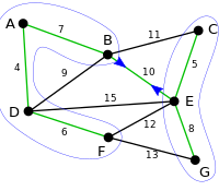
In the second and final iteration, the minimum weight edge out of each of the two remaining components is added. These happen to be the same edge. One component remains and we are done. The edge BD is not considered because both endpoints are in the same component.
763:. These randomized and deterministic algorithms combine steps of Borůvka's algorithm, reducing the number of components that remain to be connected, with steps of a different type that reduce the number of edges between pairs of components.
235:; etc. A tie-breaking rule is necessary to ensure that the created graph is indeed a forest, that is, it does not contain cycles. For example, consider a triangle graph with nodes {
1166:
131:
808:(1926). "Příspěvek k řešení otázky ekonomické stavby elektrovodních sítí (Contribution to the solution of a problem of economical construction of electrical networks)".
568:
each edge that is found to connect two vertices in the same component, so that it does not contribute to the time for searching for cheapest edges in later components.
693:
In the first iteration of the outer loop, the minimum weight edge out of every component is added. Some edges are selected twice (AD, CE). Two components remain.
632:
operations, it can be made to run in linear time, by removing all but the cheapest edge between each pair of components after each stage of the algorithm.
271:}. A tie-breaking rule which orders edges first by source, then by destination, will prevent creation of a cycle, resulting in the minimal spanning tree {
676:
This is our original weighted graph. The numbers near the edges indicate their weight. Initially, every vertex by itself is a component (blue circles).
830:; Milková, Eva; Nešetřilová, Helena (2001). "Otakar Borůvka on minimum spanning tree problem: translation of both the 1926 papers, comments, history".
1159:
1267:
731:
A faster randomized minimum spanning tree algorithm based in part on Borůvka's algorithm due to Karger, Klein, and Tarjan runs in expected
1152:
1245:
1052:
Karger, David R.; Klein, Philip N.; Tarjan, Robert E. (1995). "A randomized linear-time algorithm to find minimum spanning trees".
1007:
Bader, David A.; Cong, Guojing (2006). "Fast shared-memory algorithms for computing the minimum spanning forest of sparse graphs".
1332:
832:
231:
on vertices or edges. This can be achieved by representing vertices as integers and comparing them directly; comparing their
208:
The following pseudocode illustrates a basic implementation of Borůvka's algorithm. In the conditional clauses, every edge
37:
1250:
1322:
68:
1312:
61:
363:
and assign to each vertex its component
Initialize the cheapest edge for each component to "None"
1400:
1370:
356:
1317:
1289:
965:
827:
1196:
1405:
1360:
1327:
1208:
1113:
1061:
1016:
725:
1347:
1304:
969:
146:
51:
185:
169:
1240:
1235:
1213:
1118:
1021:
78:
1365:
1201:
1066:
721:
177:
157:
1381:
1262:
1131:
1079:
1034:
760:
193:
1337:
900:
173:
1284:
1225:
805:
779:
153:
1123:
1071:
1026:
920:
849:
841:
740:
142:
932:
863:
1188:
1175:
928:
877:
859:
699:
682:
655:
165:
71:
728:. Fast parallel algorithms can be obtained by combining Prim's algorithm with Borůvka's.
17:
1179:
961:
904:
589:
578:
232:
181:
149:
in a graph, or a minimum spanning forest in the case of a graph that is not connected.
1144:
845:
1394:
1279:
1098:
1135:
1038:
625:
1083:
188:
in 1951; and again by
Georges Sollin in 1965. This algorithm is frequently called
981:
1230:
629:
228:
1030:
587:
iterations of the outer loop until it terminates, and therefore to run in time
854:
924:
783:
1127:
1099:"A minimum spanning tree algorithm with inverse-Ackermann type complexity"
1075:
739:
time. The best known (deterministic) minimum spanning tree algorithm by
247:} and all edges of weight 1. Then a cycle could be created if we select
161:
982:"Two linear time algorithms for MST on minor closed graph classes"
1294:
1218:
1148:
908:
909:"Sur la liaison et la division des points d'un ensemble fini"
1274:
1257:
223:
If edges do not have distinct weights, then a consistent
628:, and more generally in families of graphs closed under
212:
is considered cheaper than "None". The purpose of the
81:
946:
Sollin, Georges (1965). "Le tracé de canalisation".
1346:
1303:
1187:
67:
57:
47:
125:
457:// no more trees can be merged -- we are finished
452:all components have cheapest edge set to "None"
948:Programming, Games, and Transportation Networks
880:(1938). "Étude de certains réseaux de routes".
743:is also based in part on Borůvka's and runs in
1160:
1009:Journal of Parallel and Distributed Computing
8:
479:component whose cheapest edge is not "None"
216:variable is to determine whether the forest
30:
786:[About a certain minimal problem].
1167:
1153:
1145:
964:(1999). "Spanning trees and spanners". In
720:Other algorithms for this problem include
564:As an optimization, one could remove from
445:as the cheapest edge for the component of
422:be the cheapest edge for the component of
414:as the cheapest edge for the component of
391:be the cheapest edge for the component of
36:
1117:
1065:
1020:
882:Comptes Rendus de l'Académie des Sciences
853:
576:Borůvka's algorithm can be shown to take
156:as a method of constructing an efficient
115:
107:
96:
88:
80:
27:Method for finding minimum spanning trees
639:
788:Práce Mor. Přírodověd. Spol. V Brně III
771:
29:
7:
164:. The algorithm was rediscovered by
974:Handbook of Computational Geometry
152:It was first published in 1926 by
25:
509:is "None") or (weight(
227:must be used, e.g. based on some
698:
681:
654:
251:as the minimal weight edge for {
42:Animation of Borůvka's algorithm
1382:List of graph search algorithms
549:The tie-breaking rule; returns
383:are in different components of
311:, a minimum spanning forest of
52:Minimum spanning tree algorithm
784:"O jistém problému minimálním"
126:{\displaystyle O(|E|\log |V|)}
120:
116:
108:
97:
89:
85:
1:
976:. Elsevier. pp. 425–461.
846:10.1016/S0012-365X(00)00224-7
610:is the number of vertices in
606:is the number of edges, and
292:A weighted undirected graph
1422:
1097:Chazelle, Bernard (2000).
1031:10.1016/j.jpdc.2006.06.001
761:inverse Ackermann function
315:. Initialize a forest
220:is yet a spanning forest.
1379:
645:
517:)) or (weight(
483:Add its cheapest edge to
35:
925:10.4064/cm-2-3-4-282-285
907:; Zubrzycki, S. (1951).
525:) and tie-breaking-rule(
18:Boruvka's algorithm
1290:Monte Carlo tree search
913:Colloquium Mathematicum
790:(in Czech and German).
31:Borůvka's algorithm
980:Mareš, Martin (2004).
561:in the case of a tie.
127:
1348:Minimum spanning tree
1128:10.1145/355541.355562
1076:10.1145/201019.201022
989:Archivum Mathematicum
759:time, where α is the
147:minimum spanning tree
128:
1333:Shortest path faster
1241:Breadth-first search
1236:Bidirectional search
1182:traversal algorithms
833:Discrete Mathematics
357:connected components
192:, especially in the
79:
1268:Iterative deepening
726:Kruskal's algorithm
158:electricity network
139:Borůvka's algorithm
32:
1263:Depth-first search
1054:Journal of the ACM
855:10338.dmlcz/500413
828:Nešetřil, Jaroslav
810:Elektronický Obzor
557:is preferred over
537:tie-breaking-rule(
490:is-preferred-over(
429:is-preferred-over(
398:is-preferred-over(
387:: let
194:parallel computing
190:Sollin's algorithm
168:in 1938; again by
123:
1388:
1387:
1285:Jump point search
1226:Best-first search
1015:(11): 1366–1378.
713:
712:
225:tie-breaking rule
136:
135:
16:(Redirected from
1413:
1401:Graph algorithms
1169:
1162:
1155:
1146:
1140:
1139:
1121:
1112:(6): 1028–1047.
1103:
1094:
1088:
1087:
1069:
1049:
1043:
1042:
1024:
1004:
998:
996:
986:
977:
958:
952:
951:
943:
937:
936:
919:(3–4): 282–285.
896:
890:
889:
878:Choquet, Gustave
874:
868:
867:
857:
824:
818:
817:
802:
796:
795:
776:
758:
741:Bernard Chazelle
738:
722:Prim's algorithm
716:Other algorithms
705:{A,B,C,D,E,F,G}
702:
685:
658:
640:
623:
613:
609:
605:
601:
586:
335:
328:
233:memory addresses
143:greedy algorithm
132:
130:
129:
124:
119:
111:
100:
92:
40:
33:
21:
1421:
1420:
1416:
1415:
1414:
1412:
1411:
1410:
1391:
1390:
1389:
1384:
1375:
1342:
1299:
1183:
1173:
1143:
1119:10.1.1.115.2318
1101:
1096:
1095:
1091:
1051:
1050:
1046:
1022:10.1.1.129.8991
1006:
1005:
1001:
984:
979:
962:Eppstein, David
960:
959:
955:
945:
944:
940:
905:Steinhaus, Hugo
901:Łukaszewicz, J.
898:
897:
893:
876:
875:
871:
826:
825:
821:
806:Borůvka, Otakar
804:
803:
799:
780:Borůvka, Otakar
778:
777:
773:
769:
744:
732:
718:
689:
672:
670:
668:
666:
664:
662:
638:
615:
611:
607:
603:
588:
577:
574:
562:
553:if and only if
333:
326:
206:
77:
76:
43:
28:
23:
22:
15:
12:
11:
5:
1419:
1417:
1409:
1408:
1403:
1393:
1392:
1386:
1385:
1380:
1377:
1376:
1374:
1373:
1371:Reverse-delete
1368:
1363:
1358:
1352:
1350:
1344:
1343:
1341:
1340:
1335:
1330:
1325:
1323:Floyd–Warshall
1320:
1315:
1309:
1307:
1301:
1300:
1298:
1297:
1292:
1287:
1282:
1277:
1272:
1271:
1270:
1260:
1255:
1254:
1253:
1248:
1238:
1233:
1228:
1223:
1222:
1221:
1216:
1211:
1199:
1193:
1191:
1185:
1184:
1174:
1172:
1171:
1164:
1157:
1149:
1142:
1141:
1089:
1067:10.1.1.39.9012
1060:(2): 321–328.
1044:
999:
953:
938:
903:; Perkal, J.;
891:
869:
819:
797:
770:
768:
765:
717:
714:
711:
710:
706:
703:
695:
694:
691:
686:
678:
677:
674:
659:
651:
650:
647:
644:
637:
634:
573:
570:
513:) < weight(
281:
205:
202:
154:Otakar Borůvka
145:for finding a
134:
133:
122:
118:
114:
110:
106:
103:
99:
95:
91:
87:
84:
74:
65:
64:
59:
58:Data structure
55:
54:
49:
45:
44:
41:
26:
24:
14:
13:
10:
9:
6:
4:
3:
2:
1418:
1407:
1406:Spanning tree
1404:
1402:
1399:
1398:
1396:
1383:
1378:
1372:
1369:
1367:
1364:
1362:
1359:
1357:
1354:
1353:
1351:
1349:
1345:
1339:
1336:
1334:
1331:
1329:
1326:
1324:
1321:
1319:
1316:
1314:
1311:
1310:
1308:
1306:
1305:Shortest path
1302:
1296:
1293:
1291:
1288:
1286:
1283:
1281:
1280:Fringe search
1278:
1276:
1273:
1269:
1266:
1265:
1264:
1261:
1259:
1256:
1252:
1249:
1247:
1246:Lexicographic
1244:
1243:
1242:
1239:
1237:
1234:
1232:
1229:
1227:
1224:
1220:
1217:
1215:
1212:
1210:
1207:
1206:
1205:
1204:
1200:
1198:
1195:
1194:
1192:
1190:
1186:
1181:
1177:
1170:
1165:
1163:
1158:
1156:
1151:
1150:
1147:
1137:
1133:
1129:
1125:
1120:
1115:
1111:
1107:
1100:
1093:
1090:
1085:
1081:
1077:
1073:
1068:
1063:
1059:
1055:
1048:
1045:
1040:
1036:
1032:
1028:
1023:
1018:
1014:
1010:
1003:
1000:
995:(3): 315–320.
994:
990:
983:
975:
971:
967:
963:
957:
954:
949:
942:
939:
934:
930:
926:
922:
918:
915:(in French).
914:
910:
906:
902:
895:
892:
887:
884:(in French).
883:
879:
873:
870:
865:
861:
856:
851:
847:
843:
840:(1–3): 3–36.
839:
835:
834:
829:
823:
820:
815:
811:
807:
801:
798:
793:
789:
785:
781:
775:
772:
766:
764:
762:
756:
752:
748:
742:
736:
729:
727:
723:
715:
707:
704:
701:
697:
696:
692:
687:
684:
680:
679:
675:
660:
657:
653:
652:
648:
642:
641:
635:
633:
631:
627:
626:planar graphs
622:
618:
599:
595:
591:
584:
580:
571:
569:
567:
560:
556:
552:
548:
544:
540:
536:
532:
528:
524:
520:
516:
512:
508:
504:
501:
497:
493:
489:
486:
482:
478:
475:
471:
468:
465:
461:
458:
455:
451:
448:
444:
440:
436:
432:
428:
425:
421:
417:
413:
409:
405:
401:
397:
394:
390:
386:
382:
378:
374:
370:
366:
362:
358:
354:
351:
347:
344:
340:
336:
329:
322:
318:
314:
310:
307:
303:
299:
295:
291:
288:
284:
280:
278:
274:
270:
266:
262:
258:
254:
250:
246:
242:
238:
234:
230:
226:
221:
219:
215:
211:
203:
201:
197:
195:
191:
187:
183:
179:
175:
171:
167:
163:
159:
155:
150:
148:
144:
140:
112:
104:
101:
93:
82:
75:
73:
70:
66:
63:
60:
56:
53:
50:
46:
39:
34:
19:
1355:
1313:Bellman–Ford
1202:
1109:
1105:
1092:
1057:
1053:
1047:
1012:
1008:
1002:
992:
988:
973:
956:
950:(in French).
947:
941:
916:
912:
899:Florek, K.;
894:
885:
881:
872:
837:
831:
822:
813:
812:(in Czech).
809:
800:
791:
787:
774:
754:
750:
746:
734:
730:
719:
649:Description
620:
616:
597:
593:
582:
575:
565:
563:
558:
554:
550:
546:
542:
538:
534:
530:
526:
522:
518:
514:
510:
506:
502:
499:
495:
491:
487:
484:
480:
476:
473:
469:
466:
463:
459:
456:
453:
449:
446:
442:
438:
434:
430:
426:
423:
419:
415:
411:
407:
403:
399:
395:
392:
388:
384:
380:
376:
372:
368:
364:
360:
352:
349:
345:
342:
338:
331:
324:
320:
316:
312:
308:
305:
301:
297:
293:
289:
286:
282:
276:
272:
268:
264:
260:
256:
252:
248:
244:
240:
236:
224:
222:
217:
213:
209:
207:
198:
196:literature.
189:
151:
138:
137:
1231:Beam search
1197:α–β pruning
970:Urrutia, J.
966:Sack, J.-R.
646:components
630:graph minor
521:) = weight(
229:total order
174:Łukasiewicz
72:performance
1395:Categories
1318:Dijkstra's
888:: 310–313.
816:: 153–154.
614:(assuming
572:Complexity
337:= {}.
204:Pseudocode
69:Worst-case
1361:Kruskal's
1356:Borůvka's
1328:Johnson's
1114:CiteSeerX
1062:CiteSeerX
1017:CiteSeerX
688:{A,B,D,F}
472: :=
470:completed
462: :=
460:completed
355:Find the
350:completed
341: :=
339:completed
283:algorithm
214:completed
186:Zubrzycki
182:Steinhaus
105:
1251:Parallel
972:(eds.).
794:: 37–58.
782:(1926).
690:{C,E,G}
602:, where
535:function
488:function
477:for each
375:, where
365:for each
330:) where
285:Borůvka
1136:6276962
1039:2004627
933:0048832
864:1825599
636:Example
306:output:
304:).
263:}, and
166:Choquet
162:Moravia
1366:Prim's
1189:Search
1134:
1116:
1106:J. ACM
1084:832583
1082:
1064:
1037:
1019:
931:
862:
643:Image
624:). In
503:return
290:input:
184:, and
178:Perkal
170:Florek
1338:Yen's
1176:Graph
1132:S2CID
1102:(PDF)
1080:S2CID
1035:S2CID
985:(PDF)
767:Notes
581:(log
559:edge2
555:edge1
543:edge2
539:edge1
531:edge2
527:edge1
523:edge2
519:edge1
515:edge2
511:edge1
507:edge2
496:edge2
492:edge1
474:false
367:edge
346:while
343:false
267:for {
259:for {
141:is a
62:Graph
48:Class
1295:SSS*
1219:SMA*
1214:LPA*
1209:IDA*
1180:tree
1178:and
724:and
673:{G}
596:log
551:true
467:else
464:true
454:then
441:Set
439:then
418:let
410:Set
408:then
379:and
348:not
319:to (
160:for
1124:doi
1072:doi
1027:doi
921:doi
886:206
850:hdl
842:doi
838:233
671:{F}
669:{E}
667:{D}
665:{C}
663:{B}
661:{A}
533:))
371:in
359:of
296:= (
279:}.
255:},
172:,
102:log
1397::
1275:D*
1258:B*
1203:A*
1130:.
1122:.
1110:47
1108:.
1104:.
1078:.
1070:.
1058:42
1056:.
1033:.
1025:.
1013:66
1011:.
993:40
991:.
987:.
978:;
968:;
929:MR
927:.
911:.
860:MR
858:.
848:.
836:.
814:15
757:))
749:α(
745:O(
733:O(
619:≥
547:is
545:)
541:,
529:,
500:is
498:)
494:,
485:E'
481:do
450:if
443:uv
437:)
435:yz
433:,
431:uv
427:if
420:yz
412:uv
406:)
404:wx
402:,
400:uv
396:if
389:wx
369:uv
353:do
323:,
300:,
287:is
277:bc
275:,
273:ab
265:ca
257:bc
249:ab
210:uv
180:,
176:,
1168:e
1161:t
1154:v
1138:.
1126::
1086:.
1074::
1041:.
1029::
997:.
935:.
923::
917:2
866:.
852::
844::
792:3
755:V
753:,
751:E
747:E
737:)
735:E
621:V
617:E
612:G
608:V
604:E
600:)
598:V
594:E
592:(
590:O
585:)
583:V
579:O
566:G
505:(
447:v
424:v
416:u
393:u
385:F
381:v
377:u
373:E
361:F
334:′
332:E
327:′
325:E
321:V
317:F
313:G
309:F
302:E
298:V
294:G
269:c
261:b
253:a
245:c
243:,
241:b
239:,
237:a
218:F
121:)
117:|
113:V
109:|
98:|
94:E
90:|
86:(
83:O
20:)
Text is available under the Creative Commons Attribution-ShareAlike License. Additional terms may apply.