31:
525:) that finds near-optimal (or optimal) solutions to instances of problem B, and an efficient approximation-preserving reduction from problem A to problem B, by composition we obtain an optimization algorithm that yields near-optimal solutions to instances of problem A. Approximation-preserving reductions are often used to prove
521:. Suppose we have two optimization problems such that instances of one problem can be mapped onto instances of the other, in a way that nearly optimal solutions to instances of the latter problem can be transformed back to yield nearly optimal solutions to the former. This way, if we have an optimization algorithm (or
466:
to a trivial problem, like determining if a number equals zero, by having the reduction machine solve the problem in exponential time and output zero only if there is a solution. However, this does not achieve much, because even though we can solve the new problem, performing the reduction is just as
357:
that cannot be constructed by arithmetic operations on rational numbers. Going in the other direction, however, we can certainly square a number with just one multiplication, only at the end. Using this limited form of reduction, we have shown the unsurprising result that multiplication is harder in
328:
However, the reduction becomes much harder if we add the restriction that we can only use the squaring function one time, and only at the end. In this case, even if we're allowed to use all the basic arithmetic operations, including multiplication, no reduction exists in general, because in order to
195:
First, we find ourselves trying to solve a problem that is similar to a problem we've already solved. In these cases, often a quick way of solving the new problem is to transform each instance of the new problem into instances of the old problem, solve these using our existing solution, and then use
442:
the solution to one problem, assuming the other problem is easy to solve. The many-one reduction is a stronger type of Turing reduction, and is more effective at separating problems into distinct complexity classes. However, the increased restrictions on many-one reductions make them more difficult
529:
results: if some optimization problem A is hard to approximate (under some complexity assumption) within a factor better than α for some α, and there is a β-approximation-preserving reduction from problem A to problem B, we can conclude that problem B is hard to approximate within factor α/β.
450:
for a complexity class if every problem in the class reduces to that problem, and it is also in the class itself. In this sense the problem represents the class, since any solution to it can, in combination with the reductions, be used to solve every problem in the class.
479:: "The reduction must be easy, relative to the complexity of typical problems in the class If the reduction itself were difficult to compute, an easy solution to the complete problem wouldn't necessarily yield an easy solution to the problems reducing to it."
199:
Second: suppose we have a problem that we've proven is hard to solve, and we have a similar new problem. We might suspect that it is also hard to solve. We argue by contradiction: suppose the new problem is easy to solve. Then, if we can show that
315:
320:
We also have a reduction in the other direction; obviously, if we can multiply two numbers, we can square a number. This seems to imply that these two problems are equally hard. This kind of reduction corresponds to
204:
instance of the old problem can be solved easily by transforming it into instances of the new problem and solving those, we have a contradiction. This establishes that the new problem is also hard.
216:. Suppose all we know how to do is to add, subtract, take squares, and divide by two. We can use this knowledge, combined with the following formula, to obtain the product of any two numbers:
137:, greater memory requirement, expensive need for extra hardware processor cores for a parallel solution compared to a single-threaded solution, etc.). The existence of a reduction from
355:
102:
into another problem. A sufficiently efficient reduction from one problem to another may be used to show that the second problem is at least as difficult as the first.
222:
907:
896:
885:
875:
518:
547:
we must find a reduction from a decision problem which is already known to be undecidable to P. That reduction function must be a
482:
Therefore, the appropriate notion of reduction depends on the complexity class being studied. When studying the complexity class
923:
87:
463:
35:
610:
The following example shows how to use reduction from the halting problem to prove that a language is undecidable. Suppose
870:
Thomas H. Cormen, Charles E. Leiserson, Ronald L. Rivest and
Clifford Stein, Introduction to Algorithms, MIT Press, 2001,
848:
510:
to show whether problems are or are not solvable by machines at all; in this case, reductions are restricted only to
167:
The mathematical structure generated on a set of problems by the reductions of a particular type generally forms a
133:. "Harder" means having a higher estimate of the required computational resources in a given context (e.g., higher
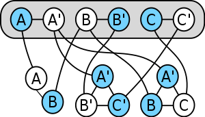
74:. The blue vertices form a minimum vertex cover, and the blue vertices in the gray oval correspond to a satisfying
833:
571:
526:
491:
422:
As described in the example above, there are two main types of reductions used in computational complexity, the
329:
get the desired result as a square we have to compute its square root first, and this square root could be an
522:
843:
853:
447:
99:
507:
487:
161:
83:
71:
880:
Hartley Rogers, Jr.: Theory of
Recursive Functions and Effective Computability, McGraw-Hill, 1967,
598:
548:
544:
511:
503:
472:
468:
379:
838:
423:
375:
359:
336:
903:
892:
881:
871:
330:
172:
157:
891:
Peter Bürgisser: Completeness and
Reduction in Algebraic Complexity Theory, Springer, 2000,
858:
540:
517:
In case of optimization (maximization or minimization) problems, we often think in terms of
427:
322:
180:
75:
156:, usually with a subscript on the ≤ to indicate the type of reduction being used (m :
590:
582:
563:
552:
499:
495:
483:
134:
623:
586:
578:
559:
411:
196:
these to obtain our final solution. This is perhaps the most obvious use of reductions.
17:
917:
176:
310:{\displaystyle a\times b={\frac {\left(\left(a+b\right)^{2}-a^{2}-b^{2}\right)}{2}}}
551:. In particular, we often show that a problem P is undecidable by showing that the
30:
459:
121:
efficiently (if it existed) could also be used as a subroutine to solve problem
641:) is the problem of determining whether the language a given Turing machine
407:
95:
371:
168:
902:
E.R. Griffor: Handbook of
Computability Theory, North Holland, 1999,
594:
567:
467:
hard as solving the old problem. Likewise, a reduction computing a
458:. For example, it's quite possible to reduce a difficult-to-solve
191:
There are two main situations where we need to use reductions:
27:
Transformation of one computational problem to another
339:
225:
633:. This language is known to be undecidable. Suppose
475:
to a decidable one. As
Michael Sipser points out in
454:However, in order to be useful, reductions must be
629:halts (by accepting or rejecting) on input string
349:
309:
684:(a Turing machine and some input string), define
494:are used. When studying classes within P such as
622:) is the problem of determining whether a given
208:A very simple example of a reduction is from
8:
732:) to check whether the language accepted by
676:(which we know does not exist). Given input
820:cannot exist, it follows that the language
720:, and does not halt otherwise. The decider
358:general than squaring. This corresponds to
145:, can be written in the shorthand notation
649:accepts any strings at all). We show that
645:accepts is empty (in other words, whether
704:that accepts only if the input string to
477:Introduction to the Theory of Computation
340:
338:
291:
278:
265:
238:
224:
792:, we would be able to produce a decider
668:. We will use this to produce a decider
125:efficiently. When this is true, solving
29:
784:can accept. Thus, if we had a decider
506:are used. Reductions are also used in
117:, if an algorithm for solving problem
7:
570:are closed under (many-one, "Karp")
418:Types and applications of reductions
660:To obtain a contradiction, suppose
653:is undecidable by a reduction from
519:approximation-preserving reduction
25:
768:, then the language accepted by
744:, then the language accepted by
34:Example of a reduction from the
696:) with the following behavior:
486:and harder classes such as the
88:computational complexity theory
464:boolean satisfiability problem
438:of another; Turing reductions
129:cannot be harder than solving
36:boolean satisfiability problem
1:
816:. Since we know that such an
849:Reduction (recursion theory)
748:is empty, so in particular
350:{\displaystyle {\sqrt {2}}}
940:
572:polynomial-time reductions
492:polynomial-time reductions
430:. Many-one reductions map
834:Gadget (computer science)
700:creates a Turing machine
527:hardness of approximation
78:for the original formula.
796:for the halting problem
177:degrees of unsolvability
752:does not halt on input
577:The complexity classes
558:The complexity classes
523:approximation algorithm
924:Reduction (complexity)
844:Parsimonious reduction
469:noncomputable function
351:
311:
175:may be used to define
79:
18:Reducible (complexity)
854:Truth table reduction
824:is also undecidable.
352:
312:
105:Intuitively, problem
98:for transforming one
33:
512:computable functions
508:computability theory
504:log-space reductions
488:polynomial hierarchy
337:
223:
162:polynomial reduction
84:computability theory
72:vertex cover problem
776:does halt on input
599:log-space reduction
549:computable function
473:undecidable problem
380:transitive relation
173:equivalence classes
839:Many-one reduction
808:) for any machine
434:of one problem to
424:many-one reduction
360:many-one reduction
347:
307:
181:complexity classes
80:
908:978-0-444-89882-1
897:978-3-540-66752-0
886:978-0-262-68052-3
876:978-0-262-03293-3
724:can now evaluate
664:is a decider for
597:are closed under
462:problem like the
370:A reduction is a
345:
331:irrational number
305:
158:mapping reduction
16:(Redirected from
931:
859:Turing reduction
772:is nonempty, so
606:Detailed example
541:decision problem
428:Turing reduction
356:
354:
353:
348:
346:
341:
323:Turing reduction
316:
314:
313:
308:
306:
301:
297:
296:
295:
283:
282:
270:
269:
264:
260:
239:
76:truth assignment
21:
939:
938:
934:
933:
932:
930:
929:
928:
914:
913:
867:
830:
760:can reject. If
716:halts on input
608:
553:halting problem
539:To show that a
536:
420:
412:natural numbers
368:
335:
334:
287:
274:
250:
246:
245:
244:
240:
221:
220:
189:
152:
135:time complexity
28:
23:
22:
15:
12:
11:
5:
937:
935:
927:
926:
916:
915:
912:
911:
900:
889:
878:
866:
863:
862:
861:
856:
851:
846:
841:
836:
829:
826:
624:Turing machine
607:
604:
603:
602:
575:
556:
535:
532:
471:can reduce an
419:
416:
367:
364:
344:
318:
317:
304:
300:
294:
290:
286:
281:
277:
273:
268:
263:
259:
256:
253:
249:
243:
237:
234:
231:
228:
210:multiplication
206:
205:
197:
188:
185:
150:
26:
24:
14:
13:
10:
9:
6:
4:
3:
2:
936:
925:
922:
921:
919:
909:
905:
901:
898:
894:
890:
887:
883:
879:
877:
873:
869:
868:
864:
860:
857:
855:
852:
850:
847:
845:
842:
840:
837:
835:
832:
831:
827:
825:
823:
819:
815:
811:
807:
803:
799:
795:
791:
787:
783:
779:
775:
771:
767:
763:
759:
755:
751:
747:
743:
739:
736:is empty. If
735:
731:
727:
723:
719:
715:
711:
707:
703:
699:
695:
691:
687:
683:
679:
675:
671:
667:
663:
658:
656:
652:
648:
644:
640:
636:
632:
628:
625:
621:
617:
613:
605:
600:
596:
592:
588:
584:
580:
576:
573:
569:
565:
561:
557:
555:reduces to P.
554:
550:
546:
542:
538:
537:
533:
531:
528:
524:
520:
515:
513:
509:
505:
501:
497:
493:
489:
485:
480:
478:
474:
470:
465:
461:
457:
452:
449:
446:A problem is
444:
441:
437:
433:
429:
425:
417:
415:
413:
409:
405:
401:
397:
393:
389:
385:
381:
377:
373:
365:
363:
361:
342:
332:
326:
324:
302:
298:
292:
288:
284:
279:
275:
271:
266:
261:
257:
254:
251:
247:
241:
235:
232:
229:
226:
219:
218:
217:
215:
211:
203:
198:
194:
193:
192:
186:
184:
182:
178:
174:
170:
165:
163:
159:
155:
148:
144:
140:
136:
132:
128:
124:
120:
116:
112:
108:
103:
101:
97:
93:
89:
85:
77:
73:
69:
65:
61:
57:
53:
49:
45:
41:
37:
32:
19:
821:
817:
813:
809:
805:
801:
797:
793:
789:
785:
781:
777:
773:
769:
765:
761:
757:
753:
749:
745:
741:
737:
733:
729:
725:
721:
717:
713:
709:
705:
701:
697:
693:
689:
685:
681:
677:
673:
669:
665:
661:
659:
654:
650:
646:
642:
638:
634:
630:
626:
619:
615:
611:
609:
516:
481:
476:
455:
453:
445:
439:
435:
431:
421:
403:
399:
395:
391:
387:
383:
374:, that is a
369:
327:
319:
213:
209:
207:
201:
190:
187:Introduction
166:
153:
146:
142:
138:
130:
126:
122:
118:
114:
110:
106:
104:
91:
81:
67:
63:
59:
55:
51:
47:
43:
39:
545:undecidable
460:NP-complete
372:preordering
160:, p :
113:to problem
865:References
812:and input
366:Properties
443:to find.
436:instances
432:instances
408:power set
406:) is the
398:), where
376:reflexive
285:−
272:−
230:×
111:reducible
96:algorithm
92:reduction
918:Category
828:See also
764:rejects
740:accepts
534:Examples
448:complete
426:and the
214:squaring
171:, whose
169:preorder
440:compute
410:of the
390:)×
100:problem
70:) to a
906:
895:
884:
874:
595:PSPACE
568:PSPACE
94:is an
58:) ∧ (¬
46:) ∧ (¬
780:, so
756:, so
543:P is
382:, on
333:like
202:every
904:ISBN
893:ISBN
882:ISBN
872:ISBN
788:for
712:and
680:and
672:for
593:and
566:and
498:and
456:easy
378:and
179:and
90:, a
86:and
708:is
212:to
164:).
141:to
109:is
82:In
54:∨ ¬
50:∨ ¬
920::
804:,
692:,
657:.
618:,
591:NP
589:,
585:,
583:NL
581:,
564:NP
562:,
514:.
502:,
500:NL
496:NC
490:,
484:NP
414:.
362:.
325:.
183:.
66:∨
62:∨
42:∨
910:.
899:.
888:.
822:E
818:S
814:w
810:M
806:w
802:M
800:(
798:H
794:S
790:E
786:R
782:S
778:w
774:M
770:N
766:N
762:R
758:S
754:w
750:M
746:N
742:N
738:R
734:N
730:N
728:(
726:R
722:S
718:w
714:M
710:w
706:N
702:N
698:S
694:w
690:M
688:(
686:S
682:w
678:M
674:H
670:S
666:E
662:R
655:H
651:E
647:M
643:M
639:M
637:(
635:E
631:w
627:M
620:w
616:M
614:(
612:H
601:.
587:P
579:L
574:.
560:P
404:N
402:(
400:P
396:N
394:(
392:P
388:N
386:(
384:P
343:2
303:2
299:)
293:2
289:b
280:2
276:a
267:2
262:)
258:b
255:+
252:a
248:(
242:(
236:=
233:b
227:a
154:B
151:m
149:≤
147:A
143:B
139:A
131:B
127:A
123:A
119:B
115:B
107:A
68:C
64:B
60:A
56:C
52:B
48:A
44:B
40:A
38:(
20:)
Text is available under the Creative Commons Attribution-ShareAlike License. Additional terms may apply.