224:
from the previous iteration, then randomly picking an x-position somewhere along the slice. By using the x-position from the previous iteration of the algorithm, in the long run we select slices with probabilities proportional to the lengths of their segments within the curve. The most difficult part of this algorithm is finding the bounds of the horizontal slice, which involves inverting the function describing the distribution being sampled from. This is especially problematic for multi-modal distributions, where the slice may consist of multiple discontinuous parts. It is often possible to use a form of rejection sampling to overcome this, where we sample from a larger slice that is known to include the desired slice in question, and then discard points outside of the desired slice. This algorithm can be used to sample from the area under
531:
78:
677:
844:, one needs to draw efficiently from all the full-conditional distributions. When sampling from a full-conditional density is not easy, a single iteration of slice sampling or the Metropolis-Hastings algorithm can be used within-Gibbs to sample from the variable in question. If the full-conditional density is log-concave, a more efficient alternative is the application of
116:
1011:
223:
The motivation here is that one way to sample a point uniformly from within an arbitrary curve is first to draw thin uniform-height horizontal slices across the whole curve. Then, we can sample a point within the curve by randomly selecting a slice that falls at or below the curve at the x-position
1373:
Next, we take a uniform sample within (−3, 3). Suppose this sample yields x = −2.9. Though this sample is within our region of interest, it does not lie within our slice (f(2.9) = ~0.08334 < 0.1), so we modify the left bound of our region of interest to this point. Now we take a uniform sample
513:
Note that, in contrast to many available methods for generating random numbers from non-uniform distributions, random variates generated directly by this approach will exhibit serial statistical dependence. In other words, not all points have the same independent likelihood of selection. This is
671:
A candidate sample is selected uniformly from within this region. If the candidate sample lies inside of the slice, then it is accepted as the new sample. If it lies outside of the slice, the candidate point becomes the new boundary for the region. A new candidate sample is taken uniformly. The
652:
In practice, sampling from a horizontal slice of a multimodal distribution is difficult. There is a tension between obtaining a large sampling region and thereby making possible large moves in the distribution space, and obtaining a simpler sampling region to increase efficiency. One option for
481:
Note that, in contrast to many available methods for generating random numbers from non-uniform distributions, random variates generated directly by this approach will exhibit serial statistical dependence. This is because to draw the next sample, we define the slice based on the value of
469:
If both the PDF and its inverse are available, and the distribution is unimodal, then finding the slice and sampling from it are simple. If not, a stepping-out procedure can be used to find a region whose endpoints fall outside the slice. Then, a sample can be drawn from the slice using
1005:
In this graphical representation of reflective sampling, the shape indicates the bounds of a sampling slice. The dots indicate start and stopping points of a sampling walk. When the samples hit the bounds of the slice, the direction of sampling is "reflected" back into the slice.
965:
To prevent random walk behavior, overrelaxation methods can be used to update each variable in turn. Overrelaxation chooses a new value on the opposite side of the mode from the current value, as opposed to choosing a new independent value from the distribution as done in Gibbs.
1199:
1880:
Damlen, P., Wakefield, J., & Walker, S. (1999). Gibbs sampling for
Bayesian non‐conjugate and hierarchical models by using auxiliary variables. Journal of the Royal Statistical Society, Series B (Statistical Methodology), 61(2),
509:
In contrast to
Metropolis, slice sampling automatically adjusts the step size to match the local shape of the density function. Implementation is arguably easier and more efficient than Gibbs sampling or simple Metropolis updates.
228:
curve, regardless of whether the function integrates to 1. In fact, scaling a function by a constant has no effect on the sampled x-positions. This means that the algorithm can be used to sample from a distribution whose
498:
Slice sampling is a Markov chain method and as such serves the same purpose as Gibbs sampling and
Metropolis. Unlike Metropolis, there is no need to manually tune the candidate function or candidate standard deviation.
534:
For a given sample x, a value for y is chosen from , which defines a "slice" of the distribution (shown by the solid horizontal line). In this case, there are two slices separated by an area outside the range of the
521:
Slice
Sampling requires that the distribution to be sampled be evaluable. One way to relax this requirement is to substitute an evaluable distribution which is proportional to the true unevaluable distribution.
1658:
865:
Single variable slice sampling can be used in the multivariate case by sampling each variable in turn repeatedly, as in Gibbs sampling. To do so requires that we can compute, for each component
1522:
960:
1080:
1260:
624:
388:
1693:
1085:
1557:
1438:
890:
806:
779:
752:
721:
341:
1225:
826:
464:
436:
412:
271:
1600:
312:
1374:
from (−2.9, 3). Suppose this time our sample yields x = 1, which is within our slice, and thus is the accepted sample output by slice sampling. Had our new
663:
value. Each endpoint of this area is tested to see if it lies outside the given slice. If not, the region is extended in the appropriate direction(s) by
680:
Finding a sample given a set of slices (the slices are represented here as blue lines and correspond to the solid line slices in the previous graph of
2101:
Meyer, Renate; Cai, Bo; Perron, François (2008-03-15). "Adaptive rejection
Metropolis sampling using Lagrange interpolation polynomials of degree 2".
1002:) are kept within the bounds of the slice by "reflecting" the direction of sampling inward toward the slice once the boundary has been hit.
514:
because to draw the next sample, we define the slice based on the value of f(x) for the current sample. However, the generated samples are
2199:
1958:
2194:
1386:
If we're interested in the peak of the distribution, we can keep repeating this process since the new point corresponds to a higher
994:
Reflective slice sampling is a technique to suppress random walk behavior in which the successive candidate samples of distribution
442:, and so on. This can be visualized as alternatively sampling the y-position and then the x-position of points under PDF, thus the
1950:
1605:
974:
This method adapts the univariate algorithm to the multivariate case by substituting a hyperrectangle for the one-dimensional
1370:
to it until it extends past the limit of the slice. After this process, the new bounds of our region of interest are (−3, 3).
1358:
Now, each endpoint of this area is tested to see if it lies outside the given slice. Our right bound lies outside our slice (
530:
33:, i.e. for drawing random samples from a statistical distribution. The method is based on the observation that to sample a
30:
344:
230:
1455:
506:
causes slow decorrelation. If the step size is too large there is great inefficiency due to a high rejection rate.
1862:
238:
23:
848:(ARS) methods. When the ARS techniques cannot be applied (since the full-conditional is non-log-concave), the
895:
645:
represents a horizontal "slice" of the distribution. The rest of each iteration is dedicated to sampling an
2018:
133:), some sampling technique must be used which takes into account the varied likelihoods for each range of
1028:
466:
values have no particular consequences or interpretations outside of their usefulness for the procedure.
87:, each value would have the same likelihood of being sampled, and your distribution would be of the form
1230:
581:
115:
1010:
2163:
only initializes the algorithm; as the algorithm progresses it will find higher and higher values of
1900:
234:
2023:
2009:
Hörmann, Wolfgang (1995-06-01). "A Rejection
Technique for Sampling from T-concave Distributions".
1403:
1022:
672:
process repeats until the candidate sample is within the slice. (See diagram for a visual example).
1194:{\displaystyle f(x)={\frac {1}{\sqrt {2\pi \cdot 3^{2}}}}\ e^{-{\frac {(x-0)^{2}}{2\cdot 3^{2}}}}}
2083:
2044:
1991:
845:
471:
111:). Instead of the original black line, your new distribution would look more like the blue line.
358:
77:
1663:
2066:; Tan, K. K. C. (1995-01-01). "Adaptive Rejection Metropolis Sampling within Gibbs Sampling".
2036:
1954:
1286:) ranges from 0 to ~0.1330, so any value between these two extremes suffice. Suppose we take
2110:
2075:
2028:
1983:
1927:
1909:
1527:
1408:
1378:
not been within our slice, we would continue the shrinking/resampling process until a valid
649:
value from the slice which is representative of the density of the region being considered.
1923:
868:
784:
757:
730:
699:
676:
1931:
1919:
1301:
which we will use to expand our region of consideration. This value is arbitrary. Suppose
515:
475:
317:
34:
1204:
1974:
Gilks, W. R.; Wild, P. (1992-01-01). "Adaptive
Rejection Sampling for Gibbs Sampling".
841:
811:
449:
421:
397:
256:
1570:
276:
2188:
2048:
518:, and are therefore expected to converge to the correct distribution in long run.
149:
Slice sampling, in its simplest form, samples uniformly from underneath the curve
37:
one can sample uniformly from the region under the graph of its density function.
2179:
503:
502:
Recall that
Metropolis is sensitive to step size. If the step size is too small
2114:
2063:
828:
is taken and accepted as the sample since it lies within the considered slice.
2040:
1914:
1895:
26:
2032:
781:
lies outside the considered slice, the region's left bound is adjusted to
2087:
2068:
Journal of the Royal
Statistical Society. Series C (Applied Statistics)
1995:
1976:
Journal of the Royal
Statistical Society. Series C (Applied Statistics)
1699:
1021:
Consider a single variable example. Suppose our true distribution is a
2079:
1987:
675:
1290:= 0.1. The problem becomes how to sample points that have values
653:
simplifying this process is regional expansion and contraction.
351:
or is at least proportional to its PDF. This defines a slice of
727:
until both endpoints are outside of the considered slice. d)
249:
Slice sampling gets its name from the first step: defining a
1366:(1) = ~0.1258 > 0.1). We expand the left bound by adding
1653:{\displaystyle \alpha ={\sqrt {-2\ln(y{\sqrt {2\pi }})}}}
1355:= 2, our current region of interest is bounded by (1, 3).
474:. Various procedures for this are described in detail by
1362:(3) = ~0.0807 < 0.1), but the left value does not (
1666:
1608:
1573:
1530:
1458:
1411:
1233:
1207:
1088:
1031:
898:
871:
814:
787:
760:
733:
702:
584:
452:
424:
418:
is sampled uniformly from this slice. A new value of
400:
361:
320:
279:
259:
157:) without the need to reject any points, as follows:
1945:
Bishop, Christopher (2006). "11.4: Slice sampling".
982:
is initialized to a random position over the slice.
390:. In other words, we are now looking at a region of
1316:from the uniform distribution within the domain of
667:
until the end both endpoints lie outside the slice.
1687:
1652:
1594:
1551:
1516:
1432:
1254:
1219:
1193:
1074:
954:
884:
820:
800:
773:
746:
715:
661:is used to define the area containing the given 'x
618:
458:
430:
406:
382:
335:
306:
265:
850:adaptive rejection Metropolis sampling algorithms
1517:{\displaystyle (0,e^{-x^{2}/2}/{\sqrt {2\pi }}]}
978:region used in the original. The hyperrectangle
754:is selected uniformly from the region. e) Since
197:Draw a horizontal line across the curve at this
45:Suppose you want to sample some random variable
1201:. The peak of the distribution is obviously at
986:is then shrunk as points from it are rejected.
125:in a manner which will retain the distribution
73:) corresponds to the likelihood at that point.
2180:http://www.probability.ca/jeff/java/slice.html
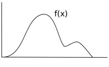
57:). Suppose that the following is the graph of
8:
2103:Computational Statistics & Data Analysis
1889:
1887:
233:is only known up to a constant (i.e. whose
103:value instead of some non-uniform function
2127:Note that if we didn't know how to select
394:where the probability density is at least
212:) from the line segments within the curve.
2143:, we can still pick any random value for
2022:
1913:
1665:
1635:
1615:
1607:
1572:
1529:
1501:
1496:
1486:
1480:
1472:
1457:
1410:
1232:
1206:
1180:
1162:
1143:
1139:
1123:
1104:
1087:
1063:
1030:
943:
924:
915:
909:
897:
876:
870:
813:
792:
786:
765:
759:
738:
732:
707:
701:
589:
583:
451:
446:s are from the desired distribution. The
423:
399:
360:
319:
278:
258:
1947:Pattern Recognition and Machine Learning
529:
1873:
567:uniformly at random from the interval ;
253:by sampling from an auxiliary variable
1025:with mean 0 and standard deviation 3,
955:{\displaystyle p(x_{i}|x_{0}...x_{n})}
1266:We first draw a uniform random value
551:) we introduce an auxiliary variable
7:
1278:) in order to define our slice(es).
861:Treating each variable independently
1308:Next, we need an initial value for
1075:{\displaystyle g(x)\sim N(0,3^{2})}
892:a function that is proportional to
696:is identified around a given point
1255:{\displaystyle f(x)\approx 0.1330}
619:{\displaystyle f^{-1}[y,+\infty )}
610:
14:
1297:Next, we set our width parameter
578:uniformly at random from the set
215:Repeat from step 2 using the new
2155:), and use that as our value of
1009:
273:. This variable is sampled from
237:is unknown), which is common in
114:
83:If you were to uniformly sample
76:
723:. c) The region is expanded by
1676:
1670:
1645:
1629:
1589:
1574:
1546:
1534:
1524:, which is bounded the pdf of
1511:
1459:
1427:
1415:
1243:
1237:
1159:
1146:
1098:
1092:
1069:
1050:
1041:
1035:
949:
916:
902:
613:
598:
371:
365:
330:
324:
301:
298:
292:
280:
183:value uniformly between 0 and
1:
1444:—say 0. After each sample of
970:Hyperrectangle slice sampling
692:is set. b) A region of width
31:pseudo-random number sampling
808:. f) Another uniform sample
633:is obtained by ignoring the
539:To sample a random variable
345:probability density function
231:probability density function
1440:we first choose an initial
1394:) than the original point.
846:adaptive rejection sampling
836:Slice-within-Gibbs sampling
2216:
2200:Non-uniform random numbers
2115:10.1016/j.csda.2008.01.005
1660:. This is the slice where
688:) ). a) A width parameter
490:) for the current sample.
383:{\displaystyle f(x)\geq Y}
1894:Neal, Radford M. (2003).
1698:An implementation in the
1688:{\displaystyle f(x)>y}
1567:uniformly at random from
1452:uniformly at random from
990:Reflective slice sampling
657:First, a width parameter
494:Compared to other methods
414:. Then the next value of
161:Choose a starting value x
2195:Markov chain Monte Carlo
1863:Markov chain Monte Carlo
1704:
1340:= 2. This works because
555:and iterate as follows:
239:computational statistics
24:Markov chain Monte Carlo
1382:within bounds is found.
1344:(2) = ~0.1065 > 0.1.
641:Our auxiliary variable
2011:ACM Trans. Math. Softw
1915:10.1214/aos/1056562461
1689:
1654:
1596:
1553:
1552:{\displaystyle N(0,1)}
1518:
1434:
1433:{\displaystyle N(0,1)}
1256:
1221:
1195:
1076:
956:
886:
829:
822:
802:
775:
748:
717:
620:
536:
460:
432:
408:
384:
337:
308:
267:
2033:10.1145/203082.203089
1690:
1655:
1597:
1554:
1519:
1435:
1257:
1222:
1196:
1077:
957:
887:
885:{\displaystyle x_{i}}
823:
803:
801:{\displaystyle x_{1}}
776:
774:{\displaystyle x_{1}}
749:
747:{\displaystyle x_{1}}
718:
716:{\displaystyle x_{0}}
679:
621:
533:
461:
433:
409:
385:
338:
309:
268:
1901:Annals of Statistics
1664:
1606:
1571:
1528:
1456:
1409:
1336:parameter). Suppose
1231:
1205:
1086:
1029:
896:
869:
856:Multivariate methods
852:are often employed.
812:
785:
758:
731:
700:
582:
450:
422:
398:
359:
336:{\displaystyle f(x)}
318:
277:
257:
235:normalizing constant
1404:normal distribution
1402:To sample from the
1220:{\displaystyle x=0}
1023:normal distribution
121:In order to sample
1685:
1650:
1592:
1549:
1514:
1430:
1324:) which satisfies
1270:from the range of
1252:
1217:
1191:
1072:
952:
882:
830:
818:
798:
771:
744:
713:
616:
537:
472:rejection sampling
456:
428:
404:
380:
333:
304:
263:
49:with distribution
1648:
1643:
1563:sample we choose
1509:
1227:, at which point
1187:
1134:
1130:
1129:
821:{\displaystyle x}
459:{\displaystyle Y}
438:is sampled, then
431:{\displaystyle Y}
407:{\displaystyle Y}
266:{\displaystyle Y}
65:). The height of
2207:
2168:
2125:
2119:
2118:
2109:(7): 3408–3423.
2098:
2092:
2091:
2059:
2053:
2052:
2026:
2006:
2000:
1999:
1971:
1965:
1964:
1942:
1936:
1935:
1917:
1896:"Slice Sampling"
1891:
1882:
1878:
1852:
1848:
1844:
1841:
1837:
1833:
1830:
1827:
1823:
1820:
1816:
1813:
1810:
1806:
1803:
1800:
1796:
1793:
1790:
1786:
1783:
1780:
1776:
1773:
1769:
1766:
1763:
1759:
1756:
1752:
1749:
1746:
1743:
1740:
1737:
1733:
1729:
1726:
1723:
1719:
1716:
1712:
1708:
1694:
1692:
1691:
1686:
1659:
1657:
1656:
1651:
1649:
1644:
1636:
1616:
1601:
1599:
1598:
1595:{\displaystyle }
1593:
1558:
1556:
1555:
1550:
1523:
1521:
1520:
1515:
1510:
1502:
1500:
1495:
1494:
1490:
1485:
1484:
1439:
1437:
1436:
1431:
1332:) > 0.1 (our
1261:
1259:
1258:
1253:
1226:
1224:
1223:
1218:
1200:
1198:
1197:
1192:
1190:
1189:
1188:
1186:
1185:
1184:
1168:
1167:
1166:
1144:
1132:
1131:
1128:
1127:
1109:
1105:
1081:
1079:
1078:
1073:
1068:
1067:
1013:
961:
959:
958:
953:
948:
947:
929:
928:
919:
914:
913:
891:
889:
888:
883:
881:
880:
827:
825:
824:
819:
807:
805:
804:
799:
797:
796:
780:
778:
777:
772:
770:
769:
753:
751:
750:
745:
743:
742:
722:
720:
719:
714:
712:
711:
625:
623:
622:
617:
597:
596:
465:
463:
462:
457:
437:
435:
434:
429:
413:
411:
410:
405:
389:
387:
386:
381:
342:
340:
339:
334:
313:
311:
310:
307:{\displaystyle }
305:
272:
270:
269:
264:
204:Sample a point (
118:
80:
2215:
2214:
2210:
2209:
2208:
2206:
2205:
2204:
2185:
2184:
2176:
2171:
2126:
2122:
2100:
2099:
2095:
2080:10.2307/2986138
2061:
2060:
2056:
2008:
2007:
2003:
1988:10.2307/2347565
1973:
1972:
1968:
1961:
1944:
1943:
1939:
1893:
1892:
1885:
1881:331-344.Chicago
1879:
1875:
1871:
1859:
1854:
1853:
1850:
1846:
1842:
1839:
1835:
1831:
1828:
1825:
1821:
1818:
1814:
1811:
1808:
1804:
1801:
1798:
1794:
1791:
1788:
1784:
1781:
1778:
1774:
1771:
1767:
1764:
1761:
1757:
1754:
1750:
1747:
1744:
1741:
1738:
1735:
1731:
1727:
1724:
1721:
1717:
1714:
1710:
1706:
1662:
1661:
1604:
1603:
1569:
1568:
1526:
1525:
1476:
1468:
1454:
1453:
1407:
1406:
1400:
1398:Another example
1229:
1228:
1203:
1202:
1176:
1169:
1158:
1145:
1135:
1119:
1084:
1083:
1059:
1027:
1026:
1019:
992:
972:
939:
920:
905:
894:
893:
872:
867:
866:
863:
858:
838:
810:
809:
788:
783:
782:
761:
756:
755:
734:
729:
728:
703:
698:
697:
585:
580:
579:
559:Given a sample
528:
526:Univariate case
496:
476:Radford M. Neal
448:
447:
420:
419:
396:
395:
357:
356:
316:
315:
275:
274:
255:
254:
247:
218:
211:
207:
200:
193:
182:
175:
164:
147:
43:
35:random variable
17:
12:
11:
5:
2213:
2211:
2203:
2202:
2197:
2187:
2186:
2183:
2182:
2175:
2174:External links
2172:
2170:
2169:
2120:
2093:
2074:(4): 455–472.
2062:Gilks, W. R.;
2054:
2024:10.1.1.56.6055
2017:(2): 182–193.
2001:
1982:(2): 337–348.
1966:
1960:978-0387310732
1959:
1937:
1908:(3): 705–767.
1883:
1872:
1870:
1867:
1866:
1865:
1858:
1855:
1705:
1684:
1681:
1678:
1675:
1672:
1669:
1647:
1642:
1639:
1634:
1631:
1628:
1625:
1622:
1619:
1614:
1611:
1591:
1588:
1585:
1582:
1579:
1576:
1548:
1545:
1542:
1539:
1536:
1533:
1513:
1508:
1505:
1499:
1493:
1489:
1483:
1479:
1475:
1471:
1467:
1464:
1461:
1429:
1426:
1423:
1420:
1417:
1414:
1399:
1396:
1384:
1383:
1371:
1356:
1345:
1306:
1295:
1251:
1248:
1245:
1242:
1239:
1236:
1216:
1213:
1210:
1183:
1179:
1175:
1172:
1165:
1161:
1157:
1154:
1151:
1148:
1142:
1138:
1126:
1122:
1118:
1115:
1112:
1108:
1103:
1100:
1097:
1094:
1091:
1071:
1066:
1062:
1058:
1055:
1052:
1049:
1046:
1043:
1040:
1037:
1034:
1018:
1015:
991:
988:
971:
968:
951:
946:
942:
938:
935:
932:
927:
923:
918:
912:
908:
904:
901:
879:
875:
862:
859:
857:
854:
837:
834:
817:
795:
791:
768:
764:
741:
737:
710:
706:
674:
673:
669:
639:
638:
629:The sample of
627:
615:
612:
609:
606:
603:
600:
595:
592:
588:
568:
527:
524:
495:
492:
455:
427:
403:
379:
376:
373:
370:
367:
364:
343:is either the
332:
329:
326:
323:
303:
300:
297:
294:
291:
288:
285:
282:
262:
246:
245:Implementation
243:
221:
220:
216:
213:
209:
205:
202:
198:
195:
191:
180:
177:
173:
162:
146:
143:
42:
39:
20:Slice sampling
15:
13:
10:
9:
6:
4:
3:
2:
2212:
2201:
2198:
2196:
2193:
2192:
2190:
2181:
2178:
2177:
2173:
2166:
2162:
2158:
2154:
2150:
2146:
2142:
2138:
2134:
2130:
2124:
2121:
2116:
2112:
2108:
2104:
2097:
2094:
2089:
2085:
2081:
2077:
2073:
2069:
2065:
2058:
2055:
2050:
2046:
2042:
2038:
2034:
2030:
2025:
2020:
2016:
2012:
2005:
2002:
1997:
1993:
1989:
1985:
1981:
1977:
1970:
1967:
1962:
1956:
1952:
1948:
1941:
1938:
1933:
1929:
1925:
1921:
1916:
1911:
1907:
1903:
1902:
1897:
1890:
1888:
1884:
1877:
1874:
1868:
1864:
1861:
1860:
1856:
1703:
1702:language is:
1701:
1696:
1682:
1679:
1673:
1667:
1640:
1637:
1632:
1626:
1623:
1620:
1617:
1612:
1609:
1586:
1583:
1580:
1577:
1566:
1562:
1559:. After each
1543:
1540:
1537:
1531:
1506:
1503:
1497:
1491:
1487:
1481:
1477:
1473:
1469:
1465:
1462:
1451:
1447:
1443:
1424:
1421:
1418:
1412:
1405:
1397:
1395:
1393:
1389:
1381:
1377:
1372:
1369:
1365:
1361:
1357:
1354:
1350:
1346:
1343:
1339:
1335:
1331:
1327:
1323:
1319:
1315:
1311:
1307:
1304:
1300:
1296:
1293:
1289:
1285:
1281:
1277:
1273:
1269:
1265:
1264:
1263:
1249:
1246:
1240:
1234:
1214:
1211:
1208:
1181:
1177:
1173:
1170:
1163:
1155:
1152:
1149:
1140:
1136:
1124:
1120:
1116:
1113:
1110:
1106:
1101:
1095:
1089:
1064:
1060:
1056:
1053:
1047:
1044:
1038:
1032:
1024:
1016:
1014:
1012:
1007:
1003:
1001:
997:
989:
987:
985:
981:
977:
969:
967:
963:
944:
940:
936:
933:
930:
925:
921:
910:
906:
899:
877:
873:
860:
855:
853:
851:
847:
843:
842:Gibbs sampler
835:
833:
815:
793:
789:
766:
762:
739:
735:
726:
708:
704:
695:
691:
687:
683:
678:
670:
668:
664:
660:
656:
655:
654:
650:
648:
644:
636:
632:
628:
607:
604:
601:
593:
590:
586:
577:
573:
569:
566:
562:
558:
557:
556:
554:
550:
546:
543:with density
542:
535:distribution.
532:
525:
523:
519:
517:
511:
507:
505:
500:
493:
491:
489:
485:
479:
477:
473:
467:
453:
445:
441:
425:
417:
401:
393:
377:
374:
368:
362:
354:
350:
346:
327:
321:
295:
289:
286:
283:
260:
252:
244:
242:
240:
236:
232:
227:
214:
203:
196:
190:
186:
178:
172:
168:
160:
159:
158:
156:
152:
144:
142:
140:
136:
132:
128:
124:
119:
117:
112:
110:
106:
102:
98:
94:
90:
86:
81:
79:
74:
72:
68:
64:
60:
56:
52:
48:
40:
38:
36:
32:
28:
25:
22:is a type of
21:
2164:
2160:
2156:
2152:
2148:
2144:
2140:
2136:
2132:
2128:
2123:
2106:
2102:
2096:
2071:
2067:
2057:
2014:
2010:
2004:
1979:
1975:
1969:
1946:
1940:
1905:
1899:
1876:
1697:
1564:
1560:
1449:
1445:
1441:
1401:
1391:
1387:
1385:
1379:
1375:
1367:
1363:
1359:
1352:
1348:
1341:
1337:
1333:
1329:
1325:
1321:
1317:
1313:
1309:
1302:
1298:
1291:
1287:
1283:
1279:
1275:
1271:
1267:
1020:
1008:
1004:
999:
995:
993:
983:
979:
975:
973:
964:
864:
849:
839:
831:
724:
693:
689:
685:
681:
666:
662:
658:
651:
646:
642:
640:
634:
630:
575:
571:
564:
560:
552:
548:
544:
540:
538:
520:
512:
508:
501:
497:
487:
483:
480:
468:
443:
439:
415:
391:
352:
348:
250:
248:
225:
222:
188:
184:
170:
166:
154:
150:
148:
138:
134:
130:
126:
122:
120:
113:
108:
104:
100:
96:
92:
88:
84:
82:
75:
70:
66:
62:
58:
54:
50:
46:
44:
19:
18:
2147:, evaluate
2064:Best, N. G.
504:random walk
2189:Categories
2131:such that
1932:1051.65007
1869:References
1448:we choose
1312:. We draw
574:we choose
563:we choose
165:for which
41:Motivation
2041:0098-3500
2019:CiteSeerX
1641:π
1627:
1618:−
1610:α
1587:α
1581:α
1578:−
1507:π
1474:−
1294:> 0.1.
1247:≈
1174:⋅
1153:−
1141:−
1117:⋅
1114:π
1045:∼
611:∞
591:−
516:markovian
375:≥
347:(PDF) of
201:position.
179:Sample a
176:) > 0.
99:for some
27:algorithm
16:Algorithm
1951:Springer
1857:See also
1351:= 2 and
1347:Because
314:, where
2139:) >
2088:2986138
1996:2347565
1924:1994729
1700:Macsyma
1017:Example
637:values.
2086:
2049:592740
2047:
2039:
2021:
1994:
1957:
1930:
1922:
1843:random
1836:random
1832:signum
1815:dfloat
1782:alpha:
1768:dfloat
1728:random
1602:where
1250:0.1330
1133:
1082:. So:
570:given
355:where
219:value.
145:Method
2084:JSTOR
2045:S2CID
1992:JSTOR
1847:alpha
1718:block
1707:slice
840:In a
251:slice
2037:ISSN
1955:ISBN
1838:())
1824:))))
1805:sqrt
1789:-2.0
1785:sqrt
1758:sqrt
1680:>
1305:= 2.
95:) =
29:for
2111:doi
2076:doi
2029:doi
1984:doi
1928:Zbl
1910:doi
1849:) )
1809:2.0
1777:)))
1762:2.0
1751:2.0
1732:exp
226:any
141:).
2191::
2159:.
2107:52
2105:.
2082:.
2072:44
2070:.
2043:.
2035:.
2027:.
2015:21
2013:.
1990:.
1980:41
1978:.
1953:.
1949:.
1926:.
1920:MR
1918:.
1906:31
1904:.
1898:.
1886:^
1829:x:
1822:pi
1795:ln
1775:pi
1753:)
1725:y:
1715::=
1713:)
1695:.
1624:ln
1262:.
962:.
832:→
478:.
241:.
208:,
194:).
2167:.
2165:y
2161:y
2157:y
2153:x
2151:(
2149:f
2145:x
2141:y
2137:x
2135:(
2133:f
2129:x
2117:.
2113::
2090:.
2078::
2051:.
2031::
1998:.
1986::
1963:.
1934:.
1912::
1851:;
1845:(
1840:*
1834:(
1826:,
1819:%
1817:(
1812:*
1807:(
1802:*
1799:y
1797:(
1792:*
1787:(
1779:,
1772:%
1770:(
1765:*
1760:(
1755:/
1748:/
1745:2
1742:^
1739:x
1736:-
1734:(
1730:(
1722:,
1720:(
1711:x
1709:(
1683:y
1677:)
1674:x
1671:(
1668:f
1646:)
1638:2
1633:y
1630:(
1621:2
1613:=
1590:]
1584:,
1575:[
1565:x
1561:y
1547:)
1544:1
1541:,
1538:0
1535:(
1532:N
1512:]
1504:2
1498:/
1492:2
1488:/
1482:2
1478:x
1470:e
1466:,
1463:0
1460:(
1450:y
1446:x
1442:x
1428:)
1425:1
1422:,
1419:0
1416:(
1413:N
1392:x
1390:(
1388:f
1380:x
1376:x
1368:w
1364:f
1360:f
1353:w
1349:x
1342:f
1338:x
1334:y
1330:x
1328:(
1326:f
1322:x
1320:(
1318:f
1314:x
1310:x
1303:w
1299:w
1292:y
1288:y
1284:x
1282:(
1280:f
1276:x
1274:(
1272:f
1268:y
1244:)
1241:x
1238:(
1235:f
1215:0
1212:=
1209:x
1182:2
1178:3
1171:2
1164:2
1160:)
1156:0
1150:x
1147:(
1137:e
1125:2
1121:3
1111:2
1107:1
1102:=
1099:)
1096:x
1093:(
1090:f
1070:)
1065:2
1061:3
1057:,
1054:0
1051:(
1048:N
1042:)
1039:x
1036:(
1033:g
1000:x
998:(
996:f
984:H
980:H
976:w
950:)
945:n
941:x
937:.
934:.
931:.
926:0
922:x
917:|
911:i
907:x
903:(
900:p
878:i
874:x
816:x
794:1
790:x
767:1
763:x
740:1
736:x
725:w
709:0
705:x
694:w
690:w
686:x
684:(
682:f
665:w
659:w
647:x
643:Y
635:y
631:x
626:.
614:)
608:+
605:,
602:y
599:[
594:1
587:f
576:x
572:y
565:y
561:x
553:Y
549:x
547:(
545:f
541:X
488:x
486:(
484:f
454:Y
444:X
440:X
426:Y
416:X
402:Y
392:X
378:Y
372:)
369:x
366:(
363:f
353:X
349:X
331:)
328:x
325:(
322:f
302:]
299:)
296:x
293:(
290:f
287:,
284:0
281:[
261:Y
217:x
210:y
206:x
199:y
192:0
189:x
187:(
185:f
181:y
174:0
171:x
169:(
167:f
163:0
155:x
153:(
151:f
139:x
137:(
135:f
131:x
129:(
127:f
123:X
109:x
107:(
105:f
101:y
97:y
93:x
91:(
89:f
85:X
71:x
69:(
67:f
63:x
61:(
59:f
55:x
53:(
51:f
47:X
Text is available under the Creative Commons Attribution-ShareAlike License. Additional terms may apply.