1307:
algorithm is needed to solve the assignment problem, and the Frank-Wolfe algorithm (with various modern modifications since first published) is used. Start with an all or nothing assignment, and then follow the rule developed by Frank-Wolfe to iterate toward the minimum value of the objective function. (The algorithm applies successive feasible solutions to achieve convergence to the optimal solution. It uses an efficient search procedure to move the calculation rapidly toward the optimal solution.) Travel times correspond to the dual variables in this programming problem.
1294:. Their work allows for feedback between congested assignment and trip distribution, although they apply sequential procedures. Starting from an initial solution of the distribution problem, the interzonal trips are assigned to the initial shortest routes. For successive iterations, new shortest routes are computed, and their lengths are used as access times for input the distribution model. The new interzonal flows are then assigned in some proportion to the routes already found. The procedure is stopped when the interzonal times for successive iteration are quasi-equal."
1097:
1086:
1075:
117:(CATS) researchers developed diversion curves for freeways versus local streets. There was much work in California also, for California had early experiences with freeway planning. In addition to work of a diversion sort, the CATS attacked some technical problems that arise when one works with complex networks. One result was the
159:
An argument can be made favoring the all-or-nothing approach. It goes this way: The planning study is to support investments so that a good level of service is available on all links. Using the travel times associated with the planned level of service, calculations indicate how traffic will flow once
1253:
refers to traffic on a link, and C is a resource constraint to be sized when fitting the model with data. Instead of using that form of the constraint, the monotonically increasing resistance function used in traffic assignment can be used. The result determines zone-to-zone movements and assigns
1132:
Disaggregate demand models were first developed to treat the mode choice problem. That problem assumes that one has decided to take a trip, where that trip will go, and at what time the trip will be made. They have been used to treat the implied broader context. Typically, a nested model will be
1115:
Figure 3 illustrates an allocation of vehicles that is not consistent with the equilibrium solution. The curves are unchanged. But with the new allocation of vehicles to routes the shaded area has to be included in the solution, so the Figure 3 solution is larger than the solution in Figure 2 by
172:
calculation procedures were developed. One heuristic proceeds incrementally. The traffic to be assigned is divided into parts (usually 4). Assign the first part of the traffic. Compute new travel times and assign the next part of the traffic. The last step is repeated until all the traffic is
1260:
A generalized disaggregate choice approach has evolved as has a generalized aggregate approach. The large question is that of the relations between them. When we use a macro model, we would like to know the disaggregate behavior it represents. If we are doing a micro analysis, we would like to
413:
conditions. The essence of these is that travelers will strive to find the shortest (least resistance) path from origin to destination, and network equilibrium occurs when no traveler can decrease travel effort by shifting to a new path. These are termed user optimal conditions, for no user will
1306:
A three link problem can not be solved graphically, and most transportation network problems involve a large numbers of nodes and links. Eash et al., for instance, studied the road net on DuPage County where there were about 30,000 one-way links and 9,500 nodes. Because problems are large, an
842:
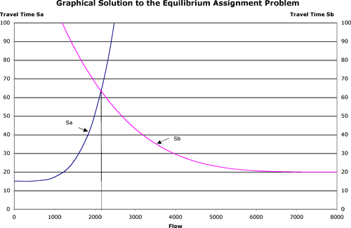
An example from Eash, Janson, and Boyce (1979) will illustrate the solution to the nonlinear program problem. There are two links from node 1 to node 2, and there is a resistance function for each link (see Figure 1). Areas under the curves in Figure 2 correspond to the integration from 0 to
105:
and expressways began to be developed. The freeway offered a superior level of service over the local street system, and diverted traffic from the local system. At first, diversion was the technique. Ratios of travel time were used, tempered by considerations of costs, comfort, and
72:. To determine facility needs and costs and benefits, we need to know the number of travelers on each route and link of the network (a route is simply a chain of links between an origin and destination). We need to undertake traffic (or trip) assignment. Suppose there is a network of
1297:
Florian et al. proposed a somewhat different method for solving the combined distribution assignment, applying directly the Frank-Wolfe algorithm. Boyce et al. (1988) summarize the research on
Network Equilibrium Problems, including the assignment with elastic demand.
1268:
with weighted parameters that say something about the attractiveness of origins and destinations. Without too much math we can write probability of choice statements based on attractiveness, and these take a form similar to some varieties of disaggregate demand models.
1310:
It is interesting that the Frank-Wolfe algorithm was available in 1956. Its application was developed in 1968, and it took almost another two decades before the first equilibrium assignment algorithm was embedded in commonly used transportation planning software
1286:
on a mathematically rigorous combination of the gravity distribution model with the equilibrium assignment model. The earliest citation of this integration is the work of Irwin and Von Cube, as related by
Florian et al. (1975), who comment on the work of Evans:
1319:, developed by Florian and others in Montreal). We would not want to draw any general conclusion from the slow application observation, mainly because we can find counter examples about the pace and pattern of technique development. For example, the
343:
1380:
has long been considered in the context of route assignment and many studies have been conducted on transit route choice. Among other factors, transit users attempt to minimize total travel time, time or distance walking, and number of transfers.
210:(1956, Florian 1976), which can be used to deal with the traffic equilibrium problem. Suppose we are considering a highway network. For each link there is a function stating the relationship between resistance and volume of traffic. The
1281:
opening where none was before inducing additional traffic has been noted for centuries. Much research has gone into developing methods for allowing the forecasting system to directly account for this phenomenon. Evans (1974) published a
1020:
935:
614:
190:
2. Now, begin to reassign using weights. Compute the weighted travel times in the previous two loadings and use those for the next assignment. The latest iteration gets a weight of 0.25 and the previous gets a weight of
1129:. In some cases, it has been noted that steps can be integrated. More generally, the steps abstract from decisions that may be made simultaneously, and it would be desirable to better replicate that in the analysis.
504:
834:= 1 if link a is on path r from i to j ; zero otherwise. So constraint (1) sums traffic on each link. There is a constraint for each link on the network. Constraint (3) assures no negative traffic.
1124:
The urban transportation planning model evolved as a set of steps to be followed, and models evolved for use in each step. Sometimes there were steps within steps, as was the case for the first statement of the
400:
There are other congestion functions. The CATS has long used a function different from that used by the BPR, but there seems to be little difference between results when the CATS and BPR functions are compared.
155:
zones, so there are numerous paths to be considered. In addition, we are ultimately interested in traffic on links. A link may be a part of several paths, and traffic along paths has to be summed link by link.
132:
and travel time increases. Absent some way to consider feedback, early planning studies (actually, most in the period 1960-1975) ignored feedback. They used the Moore algorithm to determine
740:
678:
128:
The issue the diversion approach did not handle was the feedback from the quantity of traffic on links and routes. If a lot of vehicles try to use a facility, the facility becomes
230:
832:
1067:
1524:
Eash, Ronald, Bruce N. Janson, and David Boyce
Equilibrium Trip Assignment: Advantages and Implications for Practice, Transportation Research Record 728, pp. 1–8, 1979.
1189:
1254:
traffic to networks, and that makes much sense from the way one would imagine the system works – zone-to-zone traffic depends on the resistance occasioned by congestion.
1096:
1555:
777:
1251:
1221:
1530:
Hendrickson, C.T. and B.N. Janson, "A Common
Network Flow Formulation to Several Civil Engineering Problems" Civil Engineering Systems 1(4), pp. 195–203, 1984
1518:
Dafermos, Stella. C. and F.T. Sparrow The
Traffic Assignment Problem for a General Network." J. of Res. of the National Bureau of Standards, 73B, pp. 91-118. 1969.
1085:
1527:
Evans, Suzanne P. . "Derivation and
Analysis of Some Models for Combining Trip Distribution and Assignment." Transportation Research, Vol 10, pp 37–57 1976
1347:
160:
improvements are in place. Knowing the quantities of traffic on links, the capacity to be supplied to meet the desired level of service can be calculated.
68:. The zonal interchange analysis of trip distribution provides origin-destination trip tables. Mode choice analysis tells which travelers will use which
941:
856:
514:
1257:
Alternatively, the link resistance function may be included in the objective function (and the total cost function eliminated from the constraints).
1140:
Wilson's doubly constrained entropy model has been the point of departure for efforts at the aggregate level. That model contains the constraint
1488:
Janosikova, Ludmila; Slavik, Jiri; Kohani, Michal (2014). "Estimation of a route choice model for urban public transport using smart card data".
426:
118:
1678:
1323:
for the solution of linear programming problems was worked out and widely applied prior to the development of much of programming theory.
151:
The all-or-nothing or shortest path assignment is not trivial from a technical-computational view. Each traffic zone is connected to
1673:
114:
107:
1137:
of a trip being made, then examining the choice among places, and then mode choice. The time of travel is a bit harder to treat.
1709:
1541:
1427:
Hood, Jeffrey; Sall, Elizabeth; Charlton, Billy (2011). "A GPS-based bicycle route choice model for San
Francisco, California".
211:
177:
1548:
1390:
1632:
1290:"The work of Evans resembles somewhat the algorithms developed by Irwin and Von Cube for a transportation study of
684:
1581:
1074:
53:
620:
1627:
102:
1338:
Route assignment models are based at least to some extent on empirical studies of how people choose routes in a
137:
214:(BPR) developed a link (arc) congestion (or volume-delay, or link performance) function, which we will term
1565:
338:{\displaystyle S_{a}\left({v_{a}}\right)=t_{a}\left({1+0.15\left({\frac {v_{a}}{c_{a}}}\right)^{4}}\right)}
1653:
418:
207:
133:
799:
1026:
1576:
1312:
1277:
It has long been recognized that travel demand is influenced by network supply. The example of a new
1145:
1351:
48:
concerns the selection of routes (alternatively called paths) between origins and destinations in
1637:
168:
To take account of the effect of traffic loading on travel times and traffic equilibria, several
129:
747:
1591:
1339:
1327:
410:
61:
49:
1663:
1622:
1497:
1470:
1436:
1377:
1316:
1226:
1196:
77:
1658:
1617:
1586:
57:
409:
To assign traffic to paths and links we have to have rules, and there are the well-known
1343:
1320:
173:
assigned. The CATS used a variation on this; it assigned row by row in the O-D table.
69:
1703:
1683:
1265:
122:
98:
1015:{\displaystyle S_{b}=20\left({1+0.15\left({\frac {v_{b}}{3000}}\right)^{4}}\right)}
930:{\displaystyle S_{a}=15\left({1+0.15\left({\frac {v_{a}}{1000}}\right)^{4}}\right)}
609:{\displaystyle v_{a}=\sum _{i}{\sum _{j}{\sum _{r}{\alpha _{ij}^{ar}x_{ij}^{r}}}}}
17:
1501:
1330:-– hydraulics, structures, and construction. (See Hendrickson and Janson 1984).
1688:
1668:
1596:
1533:
1455:
1440:
1134:
1126:
65:
80:
systems and a proposed addition. We first want to know the present pattern of
1474:
97:
The problem of estimating how many users are on each route is long standing.
1366:
169:
1100:
Figure 3 - Allocation of
Vehicles not Satisfying the Equilibrium Condition
1093:
Figure 3: Allocation of
Vehicles not Satisfying the Equilibrium Condition
1521:
Florian, Michael ed., Traffic
Equilibrium Methods, Springer-Verlag, 1976.
499:{\displaystyle \min \sum _{a}{\int _{0}^{v_{a}}{S_{a}\left(x\right)}}dx}
367:
per unit of time (somewhat more accurately: flow attempting to use link
30:
This article is about transport modelling. For computer networking, see
1456:"Transit Users' Route‐Choice Modelling in Transit Assignment: A Review"
1362:
1291:
81:
73:
31:
1326:
The problem statement and algorithm have general applications across
1283:
1278:
847:
in equation 1, they sum to 220,674. Note that the function for link
198:
These procedures seem to work "pretty well," but they are not exact.
1411:
1089:
Figure 2 - Graphical Solution to the Equilibrium Assignment Problem
1082:
Figure 2: Graphical Solution to the Equilibrium Assignment Problem
417:
The user optimum equilibrium can be found by solving the following
414:
gain from changing travel paths once the system is in equilibrium.
184:
0. Start by loading all traffic using an all or nothing procedure.
1416:. Institution of Civil Engineers. Vol. 1. pp. 325–378.
1537:
1095:
1084:
1073:
136:
and assigned all traffic to shortest paths. That is called
84:
delay and then what would happen if the addition were made.
791:. So constraint (2) says that all travel must take place –
187:
1. Compute the resulting travel times and reassign traffic.
180:
collection of computer programs proceeds another way.
1454:
Liu, Yulin; Bunker, Jonathan; Ferreira, Luis (2010).
1342:. Such studies are generally focused on a particular
1229:
1199:
1148:
1029:
944:
859:
802:
750:
687:
623:
517:
429:
233:
1112:. Travel time is the same on each route: about 63.
1646:
1610:
393:) is the average travel time for a vehicle on link
1245:
1215:
1183:
1061:
1014:
929:
826:
771:
734:
672:
608:
498:
337:
1413:Some Theoretical Aspects of Road Traffic Research
1261:know the aggregate implications of the analysis.
1104:At equilibrium there are 2,152 vehicles on link
430:
1273:Integrating travel demand with route assignment
735:{\displaystyle v_{a}\geq 0,\;x_{ij}^{r}\geq 0}
1549:
52:. It is the fourth step in the conventional
8:
673:{\displaystyle \sum _{r}{x_{ij}^{r}=T_{ij}}}
1556:
1542:
1534:
707:
1234:
1228:
1204:
1198:
1166:
1153:
1147:
1047:
1034:
1028:
1001:
986:
980:
965:
949:
943:
916:
901:
895:
880:
864:
858:
815:
807:
801:
763:
755:
749:
720:
712:
692:
686:
660:
647:
639:
634:
628:
622:
597:
589:
576:
568:
563:
557:
552:
546:
541:
535:
522:
516:
471:
466:
458:
453:
448:
443:
437:
428:
324:
312:
302:
296:
281:
271:
253:
248:
238:
232:
1402:
140:because either all of the traffic from
1490:Transportation Planning and Technology
1477:– via Taylor and Francis Online.
1365:have been found to prefer designated
851:is plotted in the reverse direction.
7:
1679:Public transport accessibility level
148:moves along a route or it does not.
1133:developed, say, starting with the
779:is the number of vehicles on path
25:
1674:Passengers per hour per direction
1334:Empirical Studies of Route Choice
827:{\displaystyle \alpha _{ij}^{ar}}
115:Chicago Area Transportation Study
1062:{\displaystyle v_{a}+v_{b}=8000}
352:= free flow travel time on link
1184:{\displaystyle t_{ij}c_{ij}=C}
176:The heuristic included in the
101:started looking hard at it as
1:
1391:Route choice (disambiguation)
1116:the area of the shaded area.
1633:Transit-oriented development
1502:10.1080/03081060.2014.935570
1078:Figure 1 - Two Route Network
1071:Figure 1: Two Route Network
363:= volume of traffic on link
206:Dafermos (1968) applied the
119:Bellman–Ford–Moore algorithm
1441:10.3328/TL.2011.03.01.63-75
1223:are the link travel costs,
1726:
1582:Transportation forecasting
1120:Integrating travel choices
772:{\displaystyle x_{ij}^{r}}
54:transportation forecasting
29:
1628:Green transport hierarchy
1572:
1475:10.1080/01441641003744261
1346:, and make use of either
793:i = 1 ... n; j = 1 ... n
138:all or nothing assignment
93:Long-standing techniques
1710:Transportation planning
1566:transportation planning
1410:Wardrop, J. G. (1952).
1369:and avoid steep hills.
50:transportation networks
27:Transportation networks
1429:Transportation Letters
1247:
1246:{\displaystyle t_{ij}}
1217:
1216:{\displaystyle c_{ij}}
1185:
1101:
1090:
1079:
1063:
1016:
931:
828:
773:
736:
674:
610:
500:
405:Equilibrium assignment
339:
212:Bureau of Public Roads
1654:Automobile dependency
1284:doctoral dissertation
1248:
1218:
1186:
1099:
1088:
1077:
1064:
1017:
932:
829:
774:
737:
675:
611:
501:
419:nonlinear programming
340:
208:Frank-Wolfe algorithm
202:Frank-Wolfe algorithm
1577:Land use forecasting
1227:
1197:
1146:
1027:
942:
857:
800:
748:
685:
621:
515:
427:
231:
164:Heuristic procedures
1352:revealed preference
823:
768:
725:
652:
602:
584:
465:
411:Wardrop equilibrium
378:= capacity of link
1647:Modal measurements
1638:Pedestrian village
1513:General References
1266:gravity-like model
1243:
1213:
1181:
1102:
1091:
1080:
1059:
1012:
927:
824:
803:
769:
751:
732:
708:
670:
635:
633:
606:
585:
564:
562:
551:
540:
496:
444:
442:
335:
88:General Approaches
46:traffic assignment
18:Traffic assignment
1697:
1696:
1592:Trip distribution
1463:Transport Reviews
1348:stated preference
1328:civil engineering
1264:Wilson derives a
1108:and 5847 on link
995:
910:
624:
553:
542:
531:
433:
318:
62:trip distribution
56:model, following
16:(Redirected from
1717:
1664:Cycling mobility
1623:Bicycle friendly
1602:Route assignment
1558:
1551:
1544:
1535:
1506:
1505:
1485:
1479:
1478:
1460:
1451:
1445:
1444:
1424:
1418:
1417:
1407:
1378:Public transport
1373:Public Transport
1252:
1250:
1249:
1244:
1242:
1241:
1222:
1220:
1219:
1214:
1212:
1211:
1190:
1188:
1187:
1182:
1174:
1173:
1161:
1160:
1068:
1066:
1065:
1060:
1052:
1051:
1039:
1038:
1021:
1019:
1018:
1013:
1011:
1007:
1006:
1005:
1000:
996:
991:
990:
981:
954:
953:
936:
934:
933:
928:
926:
922:
921:
920:
915:
911:
906:
905:
896:
869:
868:
833:
831:
830:
825:
822:
814:
778:
776:
775:
770:
767:
762:
741:
739:
738:
733:
724:
719:
697:
696:
679:
677:
676:
671:
669:
668:
667:
651:
646:
632:
615:
613:
612:
607:
605:
604:
603:
601:
596:
583:
575:
561:
550:
539:
527:
526:
505:
503:
502:
497:
489:
488:
487:
476:
475:
464:
463:
462:
452:
441:
382:per unit of time
356:per unit of time
344:
342:
341:
336:
334:
330:
329:
328:
323:
319:
317:
316:
307:
306:
297:
276:
275:
263:
259:
258:
257:
243:
242:
108:level of service
38:Route assignment
21:
1725:
1724:
1720:
1719:
1718:
1716:
1715:
1714:
1700:
1699:
1698:
1693:
1659:Bicycle counter
1642:
1618:Automotive city
1606:
1587:Trip generation
1568:
1562:
1515:
1510:
1509:
1487:
1486:
1482:
1458:
1453:
1452:
1448:
1426:
1425:
1421:
1409:
1408:
1404:
1399:
1387:
1375:
1360:
1336:
1304:
1275:
1230:
1225:
1224:
1200:
1195:
1194:
1162:
1149:
1144:
1143:
1122:
1043:
1030:
1025:
1024:
982:
976:
975:
961:
945:
940:
939:
897:
891:
890:
876:
860:
855:
854:
840:
798:
797:
787:to destination
746:
745:
688:
683:
682:
656:
619:
618:
518:
513:
512:
508:
477:
467:
454:
425:
424:
407:
392:
388:
377:
362:
351:
308:
298:
292:
291:
277:
267:
249:
244:
234:
229:
228:
223:
219:
204:
166:
95:
90:
58:trip generation
35:
28:
23:
22:
15:
12:
11:
5:
1723:
1721:
1713:
1712:
1702:
1701:
1695:
1694:
1692:
1691:
1686:
1681:
1676:
1671:
1666:
1661:
1656:
1650:
1648:
1644:
1643:
1641:
1640:
1635:
1630:
1625:
1620:
1614:
1612:
1611:Modes favoured
1608:
1607:
1605:
1604:
1599:
1594:
1589:
1584:
1579:
1573:
1570:
1569:
1563:
1561:
1560:
1553:
1546:
1538:
1532:
1531:
1528:
1525:
1522:
1519:
1514:
1511:
1508:
1507:
1496:(7): 638–648.
1480:
1469:(6): 753–769.
1446:
1419:
1401:
1400:
1398:
1395:
1394:
1393:
1386:
1383:
1374:
1371:
1359:
1356:
1335:
1332:
1321:simplex method
1303:
1300:
1274:
1271:
1240:
1237:
1233:
1210:
1207:
1203:
1180:
1177:
1172:
1169:
1165:
1159:
1156:
1152:
1121:
1118:
1058:
1055:
1050:
1046:
1042:
1037:
1033:
1010:
1004:
999:
994:
989:
985:
979:
974:
971:
968:
964:
960:
957:
952:
948:
925:
919:
914:
909:
904:
900:
894:
889:
886:
883:
879:
875:
872:
867:
863:
839:
836:
821:
818:
813:
810:
806:
766:
761:
758:
754:
731:
728:
723:
718:
715:
711:
706:
703:
700:
695:
691:
666:
663:
659:
655:
650:
645:
642:
638:
631:
627:
600:
595:
592:
588:
582:
579:
574:
571:
567:
560:
556:
549:
545:
538:
534:
530:
525:
521:
495:
492:
486:
483:
480:
474:
470:
461:
457:
451:
447:
440:
436:
432:
406:
403:
398:
397:
390:
386:
383:
375:
372:
360:
357:
349:
333:
327:
322:
315:
311:
305:
301:
295:
290:
287:
284:
280:
274:
270:
266:
262:
256:
252:
247:
241:
237:
221:
217:
203:
200:
196:
195:
192:
188:
185:
165:
162:
134:shortest paths
123:shortest paths
94:
91:
89:
86:
26:
24:
14:
13:
10:
9:
6:
4:
3:
2:
1722:
1711:
1708:
1707:
1705:
1690:
1687:
1685:
1684:Traffic count
1682:
1680:
1677:
1675:
1672:
1670:
1667:
1665:
1662:
1660:
1657:
1655:
1652:
1651:
1649:
1645:
1639:
1636:
1634:
1631:
1629:
1626:
1624:
1621:
1619:
1616:
1615:
1613:
1609:
1603:
1600:
1598:
1595:
1593:
1590:
1588:
1585:
1583:
1580:
1578:
1575:
1574:
1571:
1567:
1559:
1554:
1552:
1547:
1545:
1540:
1539:
1536:
1529:
1526:
1523:
1520:
1517:
1516:
1512:
1503:
1499:
1495:
1491:
1484:
1481:
1476:
1472:
1468:
1464:
1457:
1450:
1447:
1442:
1438:
1434:
1430:
1423:
1420:
1415:
1414:
1406:
1403:
1396:
1392:
1389:
1388:
1384:
1382:
1379:
1372:
1370:
1368:
1364:
1357:
1355:
1353:
1349:
1345:
1341:
1333:
1331:
1329:
1324:
1322:
1318:
1314:
1308:
1301:
1299:
1295:
1293:
1288:
1285:
1280:
1272:
1270:
1267:
1262:
1258:
1255:
1238:
1235:
1231:
1208:
1205:
1201:
1191:
1178:
1175:
1170:
1167:
1163:
1157:
1154:
1150:
1141:
1138:
1136:
1130:
1128:
1119:
1117:
1113:
1111:
1107:
1098:
1094:
1087:
1083:
1076:
1072:
1069:
1056:
1053:
1048:
1044:
1040:
1035:
1031:
1022:
1008:
1002:
997:
992:
987:
983:
977:
972:
969:
966:
962:
958:
955:
950:
946:
937:
923:
917:
912:
907:
902:
898:
892:
887:
884:
881:
877:
873:
870:
865:
861:
852:
850:
846:
837:
835:
819:
816:
811:
808:
804:
795:
794:
790:
786:
782:
764:
759:
756:
752:
742:
729:
726:
721:
716:
713:
709:
704:
701:
698:
693:
689:
680:
664:
661:
657:
653:
648:
643:
640:
636:
629:
625:
616:
598:
593:
590:
586:
580:
577:
572:
569:
565:
558:
554:
547:
543:
536:
532:
528:
523:
519:
510:
506:
493:
490:
484:
481:
478:
472:
468:
459:
455:
449:
445:
438:
434:
422:
420:
415:
412:
404:
402:
396:
384:
381:
373:
370:
366:
358:
355:
347:
346:
345:
331:
325:
320:
313:
309:
303:
299:
293:
288:
285:
282:
278:
272:
268:
264:
260:
254:
250:
245:
239:
235:
226:
225:
213:
209:
201:
199:
193:
189:
186:
183:
182:
181:
179:
174:
171:
163:
161:
157:
154:
149:
147:
143:
139:
135:
131:
126:
125:on networks.
124:
120:
116:
111:
109:
104:
100:
92:
87:
85:
83:
79:
75:
71:
67:
63:
59:
55:
51:
47:
43:
39:
33:
19:
1601:
1493:
1489:
1483:
1466:
1462:
1449:
1435:(1): 63–75.
1432:
1428:
1422:
1412:
1405:
1376:
1361:
1337:
1325:
1309:
1305:
1296:
1289:
1276:
1263:
1259:
1256:
1192:
1142:
1139:
1131:
1123:
1114:
1109:
1105:
1103:
1092:
1081:
1070:
1023:
938:
853:
848:
844:
841:
796:
792:
788:
784:
783:from origin
780:
743:
681:
617:
511:
509:subject to:
507:
423:
416:
408:
399:
394:
379:
368:
364:
353:
227:
215:
205:
197:
194:3. Continue.
175:
167:
158:
152:
150:
145:
141:
127:
121:for finding
112:
96:
45:
42:route choice
41:
37:
36:
1689:Walkability
1669:Modal share
1597:Mode choice
1135:probability
1127:Lowry model
66:mode choice
1367:bike lanes
1302:Discussion
1193:where the
805:α
727:≥
699:≥
626:∑
566:α
555:∑
544:∑
533:∑
446:∫
435:∑
170:heuristic
130:congested
1704:Category
1385:See also
1363:Cyclists
1354:models.
421:problem
103:freeways
99:Planners
74:highways
1358:Bicycle
1340:network
1292:Toronto
838:Example
82:traffic
78:transit
32:routing
1564:Urban
1317:Emme/2
1279:bridge
744:where
64:, and
1459:(PDF)
1397:Notes
191:0.75.
153:n - 1
44:, or
1344:mode
1315:and
1313:Emme
1057:8000
993:3000
973:0.15
908:1000
888:0.15
289:0.15
178:FHWA
113:The
76:and
70:mode
1498:doi
1471:doi
1437:doi
1350:or
431:min
144:to
1706::
1494:37
1492:.
1467:30
1465:.
1461:.
1431:.
959:20
874:15
389:(v
371:).
220:(v
110:.
60:,
40:,
1557:e
1550:t
1543:v
1504:.
1500::
1473::
1443:.
1439::
1433:3
1311:(
1239:j
1236:i
1232:t
1209:j
1206:i
1202:c
1179:C
1176:=
1171:j
1168:i
1164:c
1158:j
1155:i
1151:t
1110:b
1106:a
1054:=
1049:b
1045:v
1041:+
1036:a
1032:v
1009:)
1003:4
998:)
988:b
984:v
978:(
970:+
967:1
963:(
956:=
951:b
947:S
924:)
918:4
913:)
903:a
899:v
893:(
885:+
882:1
878:(
871:=
866:a
862:S
849:b
845:a
820:r
817:a
812:j
809:i
789:j
785:i
781:r
765:r
760:j
757:i
753:x
730:0
722:r
717:j
714:i
710:x
705:,
702:0
694:a
690:v
665:j
662:i
658:T
654:=
649:r
644:j
641:i
637:x
630:r
599:r
594:j
591:i
587:x
581:r
578:a
573:j
570:i
559:r
548:j
537:i
529:=
524:a
520:v
494:x
491:d
485:)
482:x
479:(
473:a
469:S
460:a
456:v
450:0
439:a
395:a
391:a
387:a
385:S
380:a
376:a
374:c
369:a
365:a
361:a
359:v
354:a
350:a
348:t
332:)
326:4
321:)
314:a
310:c
304:a
300:v
294:(
286:+
283:1
279:(
273:a
269:t
265:=
261:)
255:a
251:v
246:(
240:a
236:S
224:)
222:a
218:a
216:S
146:j
142:i
34:.
20:)
Text is available under the Creative Commons Attribution-ShareAlike License. Additional terms may apply.