Ratio of the perimeter of Bernoulli's lemniscate to its diameter
Lemniscate of Bernoulli In mathematics , the lemniscate constant ϖ is a transcendental mathematical constant that is the ratio of the perimeter of Bernoulli's lemniscate to its diameter , analogous to the definition of π
(
x
2
+
y
2
)
2
=
x
2
−
y
2
{\displaystyle (x^{2}+y^{2})^{2}=x^{2}-y^{2}}
2ϖ . The lemniscate constant is closely related to the lemniscate elliptic functions and approximately equal to 2.62205755. It also appears in evaluation of the gamma and beta function at certain rational values. The symbol ϖ is a cursive variant of π ; see Pi § Variant pi .
Sometimes the quantities 2ϖ or ϖ/2 the lemniscate constant.
As of 2024 over 1.2 trillion digits of this constant have been calculated.
History
Gauss's constant , denoted by G , is equal to ϖ /π ≈ 0.8346268Carl Friedrich Gauss , who calculated it via the arithmetic–geometric mean as
1
/
M
(
1
,
2
)
{\displaystyle 1/M{\bigl (}1,{\sqrt {2}}{\bigr )}}
M
(
1
,
2
)
=
π
/
ϖ
{\displaystyle M{\bigl (}1,{\sqrt {2}}{\bigr )}=\pi /\varpi }
ϖ
{\displaystyle \varpi }
John Todd named two more lemniscate constants, the first lemniscate constant A = ϖ /2 ≈ 1.3110287771second lemniscate constant B = π /(2ϖ ) ≈ 0.5990701173
The lemniscate constant
ϖ
{\displaystyle \varpi }
A
{\displaystyle A}
transcendental by Carl Ludwig Siegel in 1932 and later by Theodor Schneider in 1937 and Todd's second lemniscate constant
B
{\displaystyle B}
G
{\displaystyle G}
Gregory Chudnovsky proved that the set
{
π
,
ϖ
}
{\displaystyle \{\pi ,\varpi \}}
algebraically independent over
Q
{\displaystyle \mathbb {Q} }
A
{\displaystyle A}
B
{\displaystyle B}
{
π
,
M
(
1
,
1
/
2
)
,
M
′
(
1
,
1
/
2
)
}
{\displaystyle {\bigl \{}\pi ,M{\bigl (}1,1/{\sqrt {2}}{\bigr )},M'{\bigl (}1,1/{\sqrt {2}}{\bigr )}{\bigr \}}}
derivative with respect to the second variable) is not algebraically independent over
Q
{\displaystyle \mathbb {Q} }
Yuri Nesterenko proved that the set
{
π
,
ϖ
,
e
π
}
{\displaystyle \{\pi ,\varpi ,e^{\pi }\}}
Q
{\displaystyle \mathbb {Q} }
Forms
Usually,
ϖ
{\displaystyle \varpi }
ϖ
=
2
∫
0
1
d
t
1
−
t
4
=
2
∫
0
∞
d
t
1
+
t
4
=
∫
0
1
d
t
t
−
t
3
=
∫
1
∞
d
t
t
3
−
t
=
4
∫
0
∞
(
1
+
t
4
4
−
t
)
d
t
=
2
2
∫
0
1
1
−
t
4
4
d
t
=
3
∫
0
1
1
−
t
4
d
t
=
2
K
(
i
)
=
1
2
B
(
1
4
,
1
2
)
=
1
2
2
B
(
1
4
,
1
4
)
=
Γ
(
1
/
4
)
2
2
2
π
=
2
−
2
4
ζ
(
3
/
4
)
2
ζ
(
1
/
4
)
2
=
2.62205
75542
92119
81046
48395
89891
11941
…
,
{\displaystyle {\begin{aligned}\varpi &=2\int _{0}^{1}{\frac {\mathrm {d} t}{\sqrt {1-t^{4}}}}={\sqrt {2}}\int _{0}^{\infty }{\frac {\mathrm {d} t}{\sqrt {1+t^{4}}}}=\int _{0}^{1}{\frac {\mathrm {d} t}{\sqrt {t-t^{3}}}}=\int _{1}^{\infty }{\frac {\mathrm {d} t}{\sqrt {t^{3}-t}}}\\&=4\int _{0}^{\infty }{\Bigl (}{\sqrt{1+t^{4}}}-t{\Bigr )}\,\mathrm {d} t=2{\sqrt {2}}\int _{0}^{1}{\sqrt{1-t^{4}}}\mathop {\mathrm {d} t} =3\int _{0}^{1}{\sqrt {1-t^{4}}}\,\mathrm {d} t\\&=2K(i)={\tfrac {1}{2}}\mathrm {B} {\bigl (}{\tfrac {1}{4}},{\tfrac {1}{2}}{\bigr )}={\tfrac {1}{2{\sqrt {2}}}}\mathrm {B} {\bigl (}{\tfrac {1}{4}},{\tfrac {1}{4}}{\bigr )}={\frac {\Gamma (1/4)^{2}}{2{\sqrt {2\pi }}}}={\frac {2-{\sqrt {2}}}{4}}{\frac {\zeta (3/4)^{2}}{\zeta (1/4)^{2}}}\\&=2.62205\;75542\;92119\;81046\;48395\;89891\;11941\ldots ,\end{aligned}}}
where K is the complete elliptic integral of the first kind with modulus k , Β is the beta function , Γ is the gamma function and ζ is the Riemann zeta function .
The lemniscate constant can also be computed by the arithmetic–geometric mean
M
{\displaystyle M}
ϖ
=
π
M
(
1
,
2
)
.
{\displaystyle \varpi ={\frac {\pi }{M{\bigl (}1,{\sqrt {2}}{\bigr )}}}.}
Gauss's constant is typically defined as the reciprocal of the arithmetic–geometric mean of 1 and the square root of 2 , after his calculation of
M
(
1
,
2
)
{\displaystyle M{\bigl (}1,{\sqrt {2}}{\bigr )}}
G
=
1
M
(
1
,
2
)
{\displaystyle G={\frac {1}{M{\bigl (}1,{\sqrt {2}}{\bigr )}}}}
beta function B:
A
=
ϖ
2
=
1
4
B
(
1
4
,
1
2
)
,
B
=
π
2
ϖ
=
1
4
B
(
1
2
,
3
4
)
.
{\displaystyle {\begin{aligned}A&={\frac {\varpi }{2}}={\tfrac {1}{4}}\mathrm {B} {\bigl (}{\tfrac {1}{4}},{\tfrac {1}{2}}{\bigr )},\\B&={\frac {\pi }{2\varpi }}={\tfrac {1}{4}}\mathrm {B} {\bigl (}{\tfrac {1}{2}},{\tfrac {3}{4}}{\bigr )}.\end{aligned}}}
As a special value of L-functions
β
′
(
0
)
=
log
ϖ
π
{\displaystyle \beta '(0)=\log {\frac {\varpi }{\sqrt {\pi }}}}
which is analogous to
ζ
′
(
0
)
=
log
1
2
π
{\displaystyle \zeta '(0)=\log {\frac {1}{\sqrt {2\pi }}}}
where
β
{\displaystyle \beta }
Dirichlet beta function and
ζ
{\displaystyle \zeta }
Riemann zeta function .
Analogously to the Leibniz formula for π ,
β
(
1
)
=
∑
n
=
1
∞
χ
(
n
)
n
=
π
4
,
{\displaystyle \beta (1)=\sum _{n=1}^{\infty }{\frac {\chi (n)}{n}}={\frac {\pi }{4}},}
L
(
E
,
1
)
=
∑
n
=
1
∞
ν
(
n
)
n
=
ϖ
4
{\displaystyle L(E,1)=\sum _{n=1}^{\infty }{\frac {\nu (n)}{n}}={\frac {\varpi }{4}}}
L
{\displaystyle L}
L-function of the elliptic curve
E
:
y
2
=
x
3
−
x
{\displaystyle E:\,y^{2}=x^{3}-x}
Q
{\displaystyle \mathbb {Q} }
ν
{\displaystyle \nu }
multiplicative function given by
ν
(
p
n
)
=
{
p
−
N
p
,
p
∈
P
,
n
=
1
0
,
p
=
2
,
n
≥
2
ν
(
p
)
ν
(
p
n
−
1
)
−
p
ν
(
p
n
−
2
)
,
p
∈
P
∖
{
2
}
,
n
≥
2
{\displaystyle \nu (p^{n})={\begin{cases}p-{\mathcal {N}}_{p},\quad p\in \mathbb {P} ,\,n=1\\0,\quad p=2,\,n\geq 2\\\nu (p)\nu (p^{n-1})-p\nu (p^{n-2}),\quad p\in \mathbb {P} \setminus \{2\},\,n\geq 2\end{cases}}}
N
p
{\displaystyle {\mathcal {N}}_{p}}
a
3
−
a
≡
b
2
(
mod
p
)
,
p
∈
P
{\displaystyle a^{3}-a\equiv b^{2}\,(\operatorname {mod} p),\quad p\in \mathbb {P} }
a
,
b
{\displaystyle a,b}
ν
{\displaystyle \nu }
F
(
τ
)
=
η
(
4
τ
)
2
η
(
8
τ
)
2
=
∑
n
=
1
∞
ν
(
n
)
q
n
,
q
=
e
2
π
i
τ
{\displaystyle F(\tau )=\eta (4\tau )^{2}\eta (8\tau )^{2}=\sum _{n=1}^{\infty }\nu (n)q^{n},\quad q=e^{2\pi i\tau }}
τ
∈
C
{\displaystyle \tau \in \mathbb {C} }
ℑ
τ
>
0
{\displaystyle \operatorname {\Im } \tau >0}
η
{\displaystyle \eta }
eta function .
The above result can be equivalently written as
∑
n
=
1
∞
ν
(
n
)
n
e
−
2
π
n
/
32
=
ϖ
8
{\displaystyle \sum _{n=1}^{\infty }{\frac {\nu (n)}{n}}e^{-2\pi n/{\sqrt {32}}}={\frac {\varpi }{8}}}
32
{\displaystyle 32}
conductor of
E
{\displaystyle E}
BSD conjecture is true for the above
E
{\displaystyle E}
As a special value of other functions
Let
Δ
{\displaystyle \Delta }
1
{\displaystyle 1}
Δ
(
i
)
=
1
64
(
ϖ
π
)
12
.
{\displaystyle \Delta (i)={\frac {1}{64}}\left({\frac {\varpi }{\pi }}\right)^{12}.}
q
{\displaystyle q}
Δ
{\displaystyle \Delta }
Ramanujan tau function .
Series
Viète's formula for π can be written:
2
π
=
1
2
⋅
1
2
+
1
2
1
2
⋅
1
2
+
1
2
1
2
+
1
2
1
2
⋯
{\displaystyle {\frac {2}{\pi }}={\sqrt {\frac {1}{2}}}\cdot {\sqrt {{\frac {1}{2}}+{\frac {1}{2}}{\sqrt {\frac {1}{2}}}}}\cdot {\sqrt {{\frac {1}{2}}+{\frac {1}{2}}{\sqrt {{\frac {1}{2}}+{\frac {1}{2}}{\sqrt {\frac {1}{2}}}}}}}\cdots }
An analogous formula for ϖ is:
2
ϖ
=
1
2
⋅
1
2
+
1
2
/
1
2
⋅
1
2
+
1
2
/
1
2
+
1
2
/
1
2
⋯
{\displaystyle {\frac {2}{\varpi }}={\sqrt {\frac {1}{2}}}\cdot {\sqrt {{\frac {1}{2}}+{\frac {1}{2}}{\bigg /}\!{\sqrt {\frac {1}{2}}}}}\cdot {\sqrt {{\frac {1}{2}}+{\frac {1}{2}}{\Bigg /}\!{\sqrt {{\frac {1}{2}}+{\frac {1}{2}}{\bigg /}\!{\sqrt {\frac {1}{2}}}}}}}\cdots }
The Wallis product for π is:
π
2
=
∏
n
=
1
∞
(
1
+
1
n
)
(
−
1
)
n
+
1
=
∏
n
=
1
∞
(
2
n
2
n
−
1
⋅
2
n
2
n
+
1
)
=
(
2
1
⋅
2
3
)
(
4
3
⋅
4
5
)
(
6
5
⋅
6
7
)
⋯
{\displaystyle {\frac {\pi }{2}}=\prod _{n=1}^{\infty }\left(1+{\frac {1}{n}}\right)^{(-1)^{n+1}}=\prod _{n=1}^{\infty }\left({\frac {2n}{2n-1}}\cdot {\frac {2n}{2n+1}}\right)={\biggl (}{\frac {2}{1}}\cdot {\frac {2}{3}}{\biggr )}{\biggl (}{\frac {4}{3}}\cdot {\frac {4}{5}}{\biggr )}{\biggl (}{\frac {6}{5}}\cdot {\frac {6}{7}}{\biggr )}\cdots }
An analogous formula for ϖ is:
ϖ
2
=
∏
n
=
1
∞
(
1
+
1
2
n
)
(
−
1
)
n
+
1
=
∏
n
=
1
∞
(
4
n
−
1
4
n
−
2
⋅
4
n
4
n
+
1
)
=
(
3
2
⋅
4
5
)
(
7
6
⋅
8
9
)
(
11
10
⋅
12
13
)
⋯
{\displaystyle {\frac {\varpi }{2}}=\prod _{n=1}^{\infty }\left(1+{\frac {1}{2n}}\right)^{(-1)^{n+1}}=\prod _{n=1}^{\infty }\left({\frac {4n-1}{4n-2}}\cdot {\frac {4n}{4n+1}}\right)={\biggl (}{\frac {3}{2}}\cdot {\frac {4}{5}}{\biggr )}{\biggl (}{\frac {7}{6}}\cdot {\frac {8}{9}}{\biggr )}{\biggl (}{\frac {11}{10}}\cdot {\frac {12}{13}}{\biggr )}\cdots }
A related result for Gauss's constant (
G
=
ϖ
/
π
{\displaystyle G=\varpi /\pi }
ϖ
π
=
∏
n
=
1
∞
(
4
n
−
1
4
n
⋅
4
n
+
2
4
n
+
1
)
=
(
3
4
⋅
6
5
)
(
7
8
⋅
10
9
)
(
11
12
⋅
14
13
)
⋯
{\displaystyle {\frac {\varpi }{\pi }}=\prod _{n=1}^{\infty }\left({\frac {4n-1}{4n}}\cdot {\frac {4n+2}{4n+1}}\right)={\biggl (}{\frac {3}{4}}\cdot {\frac {6}{5}}{\biggr )}{\biggl (}{\frac {7}{8}}\cdot {\frac {10}{9}}{\biggr )}{\biggl (}{\frac {11}{12}}\cdot {\frac {14}{13}}{\biggr )}\cdots }
An infinite series discovered by Gauss is:
ϖ
π
=
∑
n
=
0
∞
(
−
1
)
n
∏
k
=
1
n
(
2
k
−
1
)
2
(
2
k
)
2
=
1
−
1
2
2
2
+
1
2
⋅
3
2
2
2
⋅
4
2
−
1
2
⋅
3
2
⋅
5
2
2
2
⋅
4
2
⋅
6
2
+
⋯
{\displaystyle {\frac {\varpi }{\pi }}=\sum _{n=0}^{\infty }(-1)^{n}\prod _{k=1}^{n}{\frac {(2k-1)^{2}}{(2k)^{2}}}=1-{\frac {1^{2}}{2^{2}}}+{\frac {1^{2}\cdot 3^{2}}{2^{2}\cdot 4^{2}}}-{\frac {1^{2}\cdot 3^{2}\cdot 5^{2}}{2^{2}\cdot 4^{2}\cdot 6^{2}}}+\cdots }
The Machin formula for π is
1
4
π
=
4
arctan
1
5
−
arctan
1
239
,
{\textstyle {\tfrac {1}{4}}\pi =4\arctan {\tfrac {1}{5}}-\arctan {\tfrac {1}{239}},}
π can be developed using trigonometric angle sum identities, e.g. Euler's formula
1
4
π
=
arctan
1
2
+
arctan
1
3
{\textstyle {\tfrac {1}{4}}\pi =\arctan {\tfrac {1}{2}}+\arctan {\tfrac {1}{3}}}
ϖ , including the following found by Gauss:
1
2
ϖ
=
2
arcsl
1
2
+
arcsl
7
23
{\displaystyle {\tfrac {1}{2}}\varpi =2\operatorname {arcsl} {\tfrac {1}{2}}+\operatorname {arcsl} {\tfrac {7}{23}}}
arcsl
{\displaystyle \operatorname {arcsl} }
lemniscate arcsine .
The lemniscate constant can be rapidly computed by the series
ϖ
=
2
−
1
/
2
π
(
∑
n
∈
Z
e
−
π
n
2
)
2
=
2
1
/
4
π
e
−
π
/
12
(
∑
n
∈
Z
(
−
1
)
n
e
−
π
p
n
)
2
{\displaystyle \varpi =2^{-1/2}\pi {\biggl (}\sum _{n\in \mathbb {Z} }e^{-\pi n^{2}}{\biggr )}^{2}=2^{1/4}\pi e^{-\pi /12}{\biggl (}\sum _{n\in \mathbb {Z} }(-1)^{n}e^{-\pi p_{n}}{\biggr )}^{2}}
where
p
n
=
1
2
(
3
n
2
−
n
)
{\displaystyle p_{n}={\tfrac {1}{2}}(3n^{2}-n)}
generalized pentagonal numbers ). Also
∑
m
,
n
∈
Z
e
−
2
π
(
m
2
+
m
n
+
n
2
)
=
1
+
3
ϖ
12
1
/
8
π
.
{\displaystyle \sum _{m,n\in \mathbb {Z} }e^{-2\pi (m^{2}+mn+n^{2})}={\sqrt {1+{\sqrt {3}}}}{\dfrac {\varpi }{12^{1/8}\pi }}.}
In a spirit similar to that of the Basel problem ,
∑
z
∈
Z
[
i
]
∖
{
0
}
1
z
4
=
G
4
(
i
)
=
ϖ
4
15
{\displaystyle \sum _{z\in \mathbb {Z} \setminus \{0\}}{\frac {1}{z^{4}}}=G_{4}(i)={\frac {\varpi ^{4}}{15}}}
where
Z
[
i
]
{\displaystyle \mathbb {Z} }
Gaussian integers and
G
4
{\displaystyle G_{4}}
Eisenstein series of weight
4
{\displaystyle 4}
(see Lemniscate elliptic functions § Hurwitz numbers for a more general result).
A related result is
∑
n
=
1
∞
σ
3
(
n
)
e
−
2
π
n
=
ϖ
4
80
π
4
−
1
240
{\displaystyle \sum _{n=1}^{\infty }\sigma _{3}(n)e^{-2\pi n}={\frac {\varpi ^{4}}{80\pi ^{4}}}-{\frac {1}{240}}}
where
σ
3
{\displaystyle \sigma _{3}}
sum of positive divisors function .
In 1842, Malmsten found
β
′
(
1
)
=
∑
n
=
1
∞
(
−
1
)
n
+
1
log
(
2
n
+
1
)
2
n
+
1
=
π
4
(
γ
+
2
log
π
ϖ
2
)
{\displaystyle \beta '(1)=\sum _{n=1}^{\infty }(-1)^{n+1}{\frac {\log(2n+1)}{2n+1}}={\frac {\pi }{4}}\left(\gamma +2\log {\frac {\pi }{\varpi {\sqrt {2}}}}\right)}
where
γ
{\displaystyle \gamma }
Euler's constant and
β
(
s
)
{\displaystyle \beta (s)}
The lemniscate constant is given by the rapidly converging series
ϖ
=
π
32
4
e
−
π
3
(
∑
n
=
−
∞
∞
(
−
1
)
n
e
−
2
n
π
(
3
n
+
1
)
)
2
.
{\displaystyle \varpi =\pi {\sqrt{32}}e^{-{\frac {\pi }{3}}}{\biggl (}\sum _{n=-\infty }^{\infty }(-1)^{n}e^{-2n\pi (3n+1)}{\biggr )}^{2}.}
The constant is also given by the infinite product
ϖ
=
π
∏
m
=
1
∞
tanh
2
(
π
m
2
)
.
{\displaystyle \varpi =\pi \prod _{m=1}^{\infty }\tanh ^{2}\left({\frac {\pi m}{2}}\right).}
Also
∑
n
=
0
∞
(
−
1
)
n
6635520
n
(
4
n
)
!
n
!
4
=
24
5
7
/
4
ϖ
2
π
2
.
{\displaystyle \sum _{n=0}^{\infty }{\frac {(-1)^{n}}{6635520^{n}}}{\frac {(4n)!}{n!^{4}}}={\frac {24}{5^{7/4}}}{\frac {\varpi ^{2}}{\pi ^{2}}}.}
Continued fractions
A (generalized) continued fraction for π is
π
2
=
1
+
1
1
+
1
⋅
2
1
+
2
⋅
3
1
+
3
⋅
4
1
+
⋱
{\displaystyle {\frac {\pi }{2}}=1+{\cfrac {1}{1+{\cfrac {1\cdot 2}{1+{\cfrac {2\cdot 3}{1+{\cfrac {3\cdot 4}{1+\ddots }}}}}}}}}
ϖ is
ϖ
2
=
1
+
1
2
+
2
⋅
3
2
+
4
⋅
5
2
+
6
⋅
7
2
+
⋱
{\displaystyle {\frac {\varpi }{2}}=1+{\cfrac {1}{2+{\cfrac {2\cdot 3}{2+{\cfrac {4\cdot 5}{2+{\cfrac {6\cdot 7}{2+\ddots }}}}}}}}}
Define Brouncker 's continued fraction
b
(
s
)
=
s
+
1
2
2
s
+
3
2
2
s
+
5
2
2
s
+
⋱
,
s
>
0.
{\displaystyle b(s)=s+{\cfrac {1^{2}}{2s+{\cfrac {3^{2}}{2s+{\cfrac {5^{2}}{2s+\ddots }}}}}},\quad s>0.}
n
≥
0
{\displaystyle n\geq 0}
n
≥
1
{\displaystyle n\geq 1}
b
(
4
n
)
=
(
4
n
+
1
)
∏
k
=
1
n
(
4
k
−
1
)
2
(
4
k
−
3
)
(
4
k
+
1
)
π
ϖ
2
b
(
4
n
+
1
)
=
(
2
n
+
1
)
∏
k
=
1
n
(
2
k
)
2
(
2
k
−
1
)
(
2
k
+
1
)
4
π
b
(
4
n
+
2
)
=
(
4
n
+
1
)
∏
k
=
1
n
(
4
k
−
3
)
(
4
k
+
1
)
(
4
k
−
1
)
2
ϖ
2
π
b
(
4
n
+
3
)
=
(
2
n
+
1
)
∏
k
=
1
n
(
2
k
−
1
)
(
2
k
+
1
)
(
2
k
)
2
π
.
{\displaystyle {\begin{aligned}b(4n)&=(4n+1)\prod _{k=1}^{n}{\frac {(4k-1)^{2}}{(4k-3)(4k+1)}}{\frac {\pi }{\varpi ^{2}}}\\b(4n+1)&=(2n+1)\prod _{k=1}^{n}{\frac {(2k)^{2}}{(2k-1)(2k+1)}}{\frac {4}{\pi }}\\b(4n+2)&=(4n+1)\prod _{k=1}^{n}{\frac {(4k-3)(4k+1)}{(4k-1)^{2}}}{\frac {\varpi ^{2}}{\pi }}\\b(4n+3)&=(2n+1)\prod _{k=1}^{n}{\frac {(2k-1)(2k+1)}{(2k)^{2}}}\,\pi .\end{aligned}}}
b
(
1
)
=
4
π
,
b
(
2
)
=
ϖ
2
π
,
b
(
3
)
=
π
,
b
(
4
)
=
9
π
ϖ
2
.
{\displaystyle {\begin{aligned}b(1)&={\frac {4}{\pi }},&b(2)&={\frac {\varpi ^{2}}{\pi }},&b(3)&=\pi ,&b(4)&={\frac {9\pi }{\varpi ^{2}}}.\end{aligned}}}
In fact, the values of
b
(
1
)
{\displaystyle b(1)}
b
(
2
)
{\displaystyle b(2)}
b
(
s
+
2
)
=
(
s
+
1
)
2
b
(
s
)
,
{\displaystyle b(s+2)={\frac {(s+1)^{2}}{b(s)}},}
b
(
n
)
{\displaystyle b(n)}
n
{\displaystyle n}
Simple continued fractions
Simple continued fractions for the lemniscate constant and related constants include
ϖ
=
[
2
,
1
,
1
,
1
,
1
,
1
,
4
,
1
,
2
,
…
]
,
2
ϖ
=
[
5
,
4
,
10
,
2
,
1
,
2
,
3
,
29
,
…
]
,
ϖ
2
=
[
1
,
3
,
4
,
1
,
1
,
1
,
5
,
2
,
…
]
,
ϖ
π
=
[
0
,
1
,
5
,
21
,
3
,
4
,
14
,
…
]
.
{\displaystyle {\begin{aligned}\varpi &=,\\2\varpi &=,\\{\frac {\varpi }{2}}&=,\\{\frac {\varpi }{\pi }}&=.\end{aligned}}}
Integrals
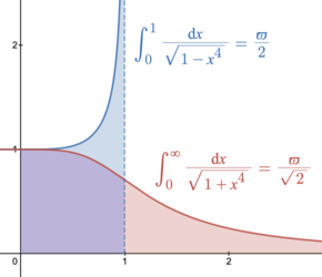
A geometric representation of
ϖ
/
2
{\displaystyle \varpi /2}
ϖ
/
2
{\displaystyle \varpi /{\sqrt {2}}}
The lemniscate constant ϖ is related to the area under the curve
x
4
+
y
4
=
1
{\displaystyle x^{4}+y^{4}=1}
π
n
:=
B
(
1
n
,
1
n
)
{\displaystyle \pi _{n}\mathrel {:=} \mathrm {B} {\bigl (}{\tfrac {1}{n}},{\tfrac {1}{n}}{\bigr )}}
x
n
+
y
n
=
1
{\displaystyle x^{n}+y^{n}=1}
2
∫
0
1
1
−
x
n
n
d
x
=
1
n
π
n
.
{\textstyle 2\int _{0}^{1}{\sqrt{1-x^{n}}}\mathop {\mathrm {d} x} ={\tfrac {1}{n}}\pi _{n}.}
1
4
π
4
=
1
2
ϖ
.
{\displaystyle {\tfrac {1}{4}}\pi _{4}={\tfrac {1}{\sqrt {2}}}\varpi .}
In 1842, Malmsten discovered that
∫
0
1
log
(
−
log
x
)
1
+
x
2
d
x
=
π
2
log
π
ϖ
2
.
{\displaystyle \int _{0}^{1}{\frac {\log(-\log x)}{1+x^{2}}}\,dx={\frac {\pi }{2}}\log {\frac {\pi }{\varpi {\sqrt {2}}}}.}
Furthermore,
∫
0
∞
tanh
x
x
e
−
x
d
x
=
log
ϖ
2
π
{\displaystyle \int _{0}^{\infty }{\frac {\tanh x}{x}}e^{-x}\,dx=\log {\frac {\varpi ^{2}}{\pi }}}
and
∫
0
∞
e
−
x
4
d
x
=
2
ϖ
2
π
4
,
analogous to
∫
0
∞
e
−
x
2
d
x
=
π
2
,
{\displaystyle \int _{0}^{\infty }e^{-x^{4}}\,dx={\frac {\sqrt {2\varpi {\sqrt {2\pi }}}}{4}},\quad {\text{analogous to}}\,\int _{0}^{\infty }e^{-x^{2}}\,dx={\frac {\sqrt {\pi }}{2}},}
Gaussian integral .
The lemniscate constant appears in the evaluation of the integrals
π
ϖ
=
∫
0
π
2
sin
(
x
)
d
x
=
∫
0
π
2
cos
(
x
)
d
x
{\displaystyle {\frac {\pi }{\varpi }}=\int _{0}^{\frac {\pi }{2}}{\sqrt {\sin(x)}}\,dx=\int _{0}^{\frac {\pi }{2}}{\sqrt {\cos(x)}}\,dx}
ϖ
π
=
∫
0
∞
d
x
cosh
(
π
x
)
{\displaystyle {\frac {\varpi }{\pi }}=\int _{0}^{\infty }{\frac {dx}{\sqrt {\cosh(\pi x)}}}}
John Todd's lemniscate constants are defined by integrals:
A
=
∫
0
1
d
x
1
−
x
4
{\displaystyle A=\int _{0}^{1}{\frac {dx}{\sqrt {1-x^{4}}}}}
B
=
∫
0
1
x
2
d
x
1
−
x
4
{\displaystyle B=\int _{0}^{1}{\frac {x^{2}\,dx}{\sqrt {1-x^{4}}}}}
Circumference of an ellipse
The lemniscate constant satisfies the equation
π
ϖ
=
2
∫
0
1
x
2
d
x
1
−
x
4
{\displaystyle {\frac {\pi }{\varpi }}=2\int _{0}^{1}{\frac {x^{2}\,dx}{\sqrt {1-x^{4}}}}}
Euler discovered in 1738 that for the rectangular elastica (first and second lemniscate constants)
arc
length
⋅
height
=
A
⋅
B
=
∫
0
1
d
x
1
−
x
4
⋅
∫
0
1
x
2
d
x
1
−
x
4
=
ϖ
2
⋅
π
2
ϖ
=
π
4
{\displaystyle {\textrm {arc}}\ {\textrm {length}}\cdot {\textrm {height}}=A\cdot B=\int _{0}^{1}{\frac {\mathrm {d} x}{\sqrt {1-x^{4}}}}\cdot \int _{0}^{1}{\frac {x^{2}\mathop {\mathrm {d} x} }{\sqrt {1-x^{4}}}}={\frac {\varpi }{2}}\cdot {\frac {\pi }{2\varpi }}={\frac {\pi }{4}}}
Now considering the circumference
C
{\displaystyle C}
2
{\displaystyle {\sqrt {2}}}
1
{\displaystyle 1}
2
x
2
+
4
y
2
=
1
{\displaystyle 2x^{2}+4y^{2}=1}
C
2
=
∫
0
1
d
x
1
−
x
4
+
∫
0
1
x
2
d
x
1
−
x
4
{\displaystyle {\frac {C}{2}}=\int _{0}^{1}{\frac {dx}{\sqrt {1-x^{4}}}}+\int _{0}^{1}{\frac {x^{2}\,dx}{\sqrt {1-x^{4}}}}}
Hence the full circumference is
C
=
π
ϖ
+
ϖ
=
3.820197789
…
{\displaystyle C={\frac {\pi }{\varpi }}+\varpi =3.820197789\ldots }
This is also the arc length of the sine curve on half a period:
C
=
∫
0
π
1
+
cos
2
(
x
)
d
x
{\displaystyle C=\int _{0}^{\pi }{\sqrt {1+\cos ^{2}(x)}}\,dx}
Other limits
Analogously to
2
π
=
lim
n
→
∞
|
(
2
n
)
!
B
2
n
|
1
2
n
{\displaystyle 2\pi =\lim _{n\to \infty }\left|{\frac {(2n)!}{\mathrm {B} _{2n}}}\right|^{\frac {1}{2n}}}
B
n
{\displaystyle \mathrm {B} _{n}}
Bernoulli numbers , we have
2
ϖ
=
lim
n
→
∞
(
(
4
n
)
!
H
4
n
)
1
4
n
{\displaystyle 2\varpi =\lim _{n\to \infty }\left({\frac {(4n)!}{\mathrm {H} _{4n}}}\right)^{\frac {1}{4n}}}
H
n
{\displaystyle \mathrm {H} _{n}}
Hurwitz numbers .
Notes
See:
See:
Finch 2003 , p. 420Kobayashi, Hiroyuki; Takeuchi, Shingo (2019), "Applications of generalized trigonometric functions with two parameters", Communications on Pure & Applied Analysis , 18 (3): 1509–1521, arXiv :1903.07407 doi :10.3934/cpaa.2019072 , S2CID 102487670 Asai, Tetsuya (2007), Elliptic Gauss Sums and Hecke L-values at s=1 , arXiv :0707.3711 "A062539 - Oeis" . "A064853 - Oeis" ."Lemniscate Constant" ."Records set by y-cruncher" . numberworld.org . Retrieved 2024-08-20 ."A014549 - Oeis" .Finch 2003 , p. 420.Neither of these proofs was rigorous from the modern point of view. See Cox 1984 , p. 281
^ Todd, John (January 1975). "The lemniscate constants" . Communications of the ACM 18 (1): 14–19. doi :10.1145/360569.360580 S2CID 85873 . ^ "A085565 - Oeis" ."A076390 - Oeis" .Carlson, B. C. (2010), "Elliptic Integrals" , in Olver, Frank W. J. ; Lozier, Daniel M.; Boisvert, Ronald F.; Clark, Charles W. (eds.), NIST Handbook of Mathematical Functions ISBN 978-0-521-19225-5 MR 2723248 . In particular, Siegel proved that if
G
4
(
ω
1
,
ω
2
)
{\displaystyle \operatorname {G} _{4}(\omega _{1},\omega _{2})}
G
6
(
ω
1
,
ω
2
)
{\displaystyle \operatorname {G} _{6}(\omega _{1},\omega _{2})}
Im
(
ω
2
/
ω
1
)
>
0
{\displaystyle \operatorname {Im} (\omega _{2}/\omega _{1})>0}
ω
1
{\displaystyle \omega _{1}}
ω
2
{\displaystyle \omega _{2}}
G
4
{\displaystyle \operatorname {G} _{4}}
G
6
{\displaystyle \operatorname {G} _{6}}
Eisenstein series . The fact that
ϖ
{\displaystyle \varpi }
G
4
(
ϖ
,
ϖ
i
)
=
1
/
15
{\displaystyle \operatorname {G} _{4}(\varpi ,\varpi i)=1/15}
G
6
(
ϖ
,
ϖ
i
)
=
0.
{\displaystyle \operatorname {G} _{6}(\varpi ,\varpi i)=0.}
Apostol, T. M. (1990). Modular Functions and Dirichlet Series in Number Theory (Second ed.). Springer. p. 12. ISBN 0-387-97127-0 Siegel, C. L. (1932). "Über die Perioden elliptischer Funktionen" . Journal für die reine und angewandte Mathematik 167 : 62–69.
In particular, Schneider proved that the beta function
B
(
a
,
b
)
{\displaystyle \mathrm {B} (a,b)}
a
,
b
∈
Q
∖
Z
{\displaystyle a,b\in \mathbb {Q} \setminus \mathbb {Z} }
a
+
b
∉
Z
0
−
{\displaystyle a+b\notin \mathbb {Z} _{0}^{-}}
ϖ
{\displaystyle \varpi }
ϖ
=
1
2
B
(
1
4
,
1
2
)
{\displaystyle \varpi ={\tfrac {1}{2}}\mathrm {B} {\bigl (}{\tfrac {1}{4}},{\tfrac {1}{2}}{\bigr )}}
B and G from
B
(
1
2
,
3
4
)
.
{\displaystyle \mathrm {B} {\bigl (}{\tfrac {1}{2}},{\tfrac {3}{4}}{\bigr )}.}
Schneider, Theodor (1941). "Zur Theorie der Abelschen Funktionen und Integrale" . Journal für die reine und angewandte Mathematik . 183 (19): 110–128. doi :10.1515/crll.1941.183.110 . S2CID 118624331 .
G. V. Choodnovsky: Algebraic independence of constants connected with the functions of analysis , Notices of the AMS 22, 1975, p. A-486
G. V. Chudnovsky: Contributions to The Theory of Transcendental Numbers , American Mathematical Society, 1984, p. 6
In fact,
π
=
2
2
M
3
(
1
,
1
2
)
M
′
(
1
,
1
2
)
=
1
G
3
M
′
(
1
,
1
2
)
.
{\displaystyle \pi =2{\sqrt {2}}{\frac {M^{3}\left(1,{\frac {1}{\sqrt {2}}}\right)}{M'\left(1,{\frac {1}{\sqrt {2}}}\right)}}={\frac {1}{G^{3}M'\left(1,{\frac {1}{\sqrt {2}}}\right)}}.}
Borwein, Jonathan M.; Borwein, Peter B. (1987). Pi and the AGM: A Study in Analytic Number Theory and Computational Complexity (First ed.). Wiley-Interscience. ISBN 0-471-83138-7 p. 45
Nesterenko, Y. V.; Philippon, P. (2001). Introduction to Algebraic Independence Theory . Springer. p. 27. ISBN 3-540-41496-7 See:
Cox 1984 , p. 277."A113847 - Oeis" .Cremona, J. E. (1997). Algorithms for Modular Elliptic Curves Cambridge University Press . ISBN 0521598206 p. 31, formula (2.8.10)In fact, the series
∑
n
=
1
∞
ν
(
n
)
n
s
{\textstyle \sum _{n=1}^{\infty }{\frac {\nu (n)}{n^{s}}}}
ℜ
s
>
5
/
6
{\displaystyle \operatorname {\Re } s>5/6}
Murty, Vijaya Kumar (1995). Seminar on Fermat's Last Theorem . American Mathematical Society . p. 16. ISBN 9780821803134 Cohen, Henri (1993). A Course in Computational Algebraic Number Theory . Springer-Verlag. p. 382–406. ISBN 978-3-642-08142-2 "Elliptic curve with LMFDB label 32.a3 (Cremona label 32a2)" . The L-functions and modular forms database .The function
F
{\displaystyle F}
2
{\displaystyle 2}
32
{\displaystyle 32}
new form and it satisfies the functional equation
F
(
−
1
τ
)
=
−
τ
2
32
F
(
τ
1
32
)
.
{\displaystyle F\left(-{\frac {1}{\tau }}\right)=-{\frac {\tau ^{2}}{32}}F\left({\frac {\tau {\vphantom {1}}}{32}}\right).}
The
ν
{\displaystyle \nu }
ξ
{\displaystyle \xi }
ξ
(
p
n
)
=
{
1
,
p
=
2
n
+
1
,
p
∈
P
,
p
≡
1
(
mod
4
)
mod
(
n
+
1
,
2
)
,
p
∈
P
,
p
≡
3
(
mod
4
)
{\displaystyle \xi (p^{n})={\begin{cases}1,\quad p=2\\n+1,\quad p\in \mathbb {P} ,\,p\equiv 1\,(\operatorname {mod} 4)\\\operatorname {mod} (n+1,2),\quad p\in \mathbb {P} ,\,p\equiv 3\,(\operatorname {mod} 4)\end{cases}}}
n
{\displaystyle n}
ξ
{\displaystyle \xi }
Dirichlet character from the Leibniz formula for π by
∑
d
|
n
χ
(
d
)
=
ξ
(
n
)
{\displaystyle \sum _{d|n}\chi (d)=\xi (n)}
n
{\displaystyle n}
ν
{\displaystyle \nu }
ξ
{\displaystyle \xi }
∑
k
=
0
n
(
−
1
)
k
ξ
(
4
k
+
1
)
ξ
(
4
n
−
4
k
+
1
)
=
ν
(
2
n
+
1
)
{\displaystyle \sum _{k=0}^{n}(-1)^{k}\xi (4k+1)\xi (4n-4k+1)=\nu (2n+1)}
n
{\displaystyle n}
The
ν
{\displaystyle \nu }
∑
z
∈
G
;
z
z
¯
=
n
z
=
ν
(
n
)
{\displaystyle \sum _{z\in \mathbb {G} ;\,z{\overline {z}}=n}z=\nu (n)}
n
{\displaystyle n}
G
{\displaystyle \operatorname {\mathbb {G} } }
Gaussian integers of the form
(
−
1
)
a
±
b
−
1
2
(
a
±
b
i
)
{\displaystyle (-1)^{\frac {a\pm b-1}{2}}(a\pm bi)}
a
{\displaystyle a}
b
{\displaystyle b}
Rubin, Karl (1987). "Tate-Shafarevich groups and L-functions of elliptic curves with complex multiplication" . Inventiones mathematicae . 89 : 528. "Newform orbit 1.12.a.a" . The L-functions and modular forms database .Levin (2006)
Hyde (2014) proves the validity of a more general Wallis-like formula for clover curves; here the special case of the lemniscate is slightly transformed, for clarity.
Hyde, Trevor (2014). "A Wallis product on clovers" (PDF) . The American Mathematical Monthly . 121 (3): 237–243. doi :10.4169/amer.math.monthly.121.03.237 . S2CID 34819500 . Bottazzini, Umberto ; Gray, Jeremy (2013). Hidden Harmony – Geometric Fantasies: The Rise of Complex Function Theory . Springer. doi :10.1007/978-1-4614-5725-1 . ISBN 978-1-4614-5724-4 Todd (1975)
Cox 1984 , p. 307, eq. 2.21 for the first equality. The second equality can be proved by using the pentagonal number theorem .Berndt, Bruce C. (1998). Ramanujan's Notebooks Part V . Springer. ISBN 978-1-4612-7221-2 p. 326This formula can be proved by hypergeometric inversion : Let
a
(
q
)
=
∑
m
,
n
∈
Z
q
m
2
+
m
n
+
n
2
{\displaystyle \operatorname {a} (q)=\sum _{m,n\in \mathbb {Z} }q^{m^{2}+mn+n^{2}}}
q
∈
C
{\displaystyle q\in \mathbb {C} }
|
q
|
<
1
{\displaystyle \left|q\right|<1}
a
(
q
)
=
2
F
1
(
1
3
,
2
3
,
1
,
z
)
{\displaystyle \operatorname {a} (q)={}_{2}F_{1}\left({\frac {1}{3}},{\frac {2}{3}},1,z\right)}
q
=
exp
(
−
2
π
3
2
F
1
(
1
/
3
,
2
/
3
,
1
,
1
−
z
)
2
F
1
(
1
/
3
,
2
/
3
,
1
,
z
)
)
{\displaystyle q=\exp \left(-{\frac {2\pi }{\sqrt {3}}}{\frac {{}_{2}F_{1}(1/3,2/3,1,1-z)}{{}_{2}F_{1}(1/3,2/3,1,z)}}\right)}
z
∈
C
∖
{
0
,
1
}
{\displaystyle z\in \mathbb {C} \setminus \{0,1\}}
z
=
1
4
(
3
3
−
5
)
{\textstyle z={\tfrac {1}{4}}{\bigl (}3{\sqrt {3}}-5{\bigr )}}
Eymard, Pierre; Lafon, Jean-Pierre (2004). The Number Pi . American Mathematical Society. ISBN 0-8218-3246-8 p. 232Garrett, Paul. "Level-one elliptic modular forms" (PDF) . University of Minnesota . p. 11—13The formula follows from the hypergeometric transformation
3
F
2
(
1
4
,
1
2
,
3
4
,
1
,
1
,
16
z
(
1
−
z
)
2
(
1
+
z
)
4
)
=
(
1
+
z
)
2
F
1
(
1
2
,
1
2
,
1
,
z
)
2
{\displaystyle {}_{3}F_{2}\left({\frac {1}{4}},{\frac {1}{2}},{\frac {3}{4}},1,1,16z{\frac {(1-z)^{2}}{(1+z)^{4}}}\right)=(1+z)\,{}_{2}F_{1}\left({\frac {1}{2}},{\frac {1}{2}},1,z\right)^{2}}
z
=
λ
(
1
+
5
i
)
{\displaystyle z=\lambda (1+5i)}
λ
{\displaystyle \lambda }
modular lambda function .
Khrushchev, Sergey (2008). Orthogonal Polynomials and Continued Fractions (First ed.). Cambridge University Press. ISBN 978-0-521-85419-1 p. 140 (eq. 3.34), p. 153. There's an error on p. 153:
4
[
Γ
(
3
+
s
/
4
)
/
Γ
(
1
+
s
/
4
)
]
2
{\displaystyle 4^{2}}
4
[
Γ
(
(
3
+
s
)
/
4
)
/
Γ
(
(
1
+
s
)
/
4
)
]
2
{\displaystyle 4^{2}}
Khrushchev, Sergey (2008). Orthogonal Polynomials and Continued Fractions (First ed.). Cambridge University Press. ISBN 978-0-521-85419-1 p. 146, 155Perron, Oskar (1957). Die Lehre von den Kettenbrüchen: Band II (in German) (Third ed.). B. G. Teubner."A062540 - OEIS" . oeis.org . Retrieved 2022-09-14 ."A053002 - OEIS" . oeis.org .Blagouchine, Iaroslav V. (2014). "Rediscovery of Malmsten's integrals, their evaluation by contour integration methods and some related results" . The Ramanujan Journal . 35 (1): 21–110. doi :10.1007/s11139-013-9528-5 . S2CID 120943474 . "A068467 - Oeis" .^ Cox 1984 , p. 313.Levien (2008)
Cox 1984 , p. 312.Adlaj, Semjon (2012). "An Eloquent Formula for the Perimeter of an Ellipse" (PDF) . American Mathematical Society . p. 1097. One might also observe that the length of the "sine" curve over half a period, that is, the length of the graph of the function sin(t) from the point where t = 0 to the point where t = π , is
2
l
(
1
/
2
)
=
L
+
M
{\displaystyle {\sqrt {2}}l(1/{\sqrt {2}})=L+M}
In this paper
M
=
1
/
G
=
π
/
ϖ
{\displaystyle M=1/G=\pi /\varpi }
L
=
π
/
M
=
G
π
=
ϖ
{\displaystyle L=\pi /M=G\pi =\varpi }
References
External links